Exploratory Data Analysis Part 3 - What Makes the Difference Between the Two

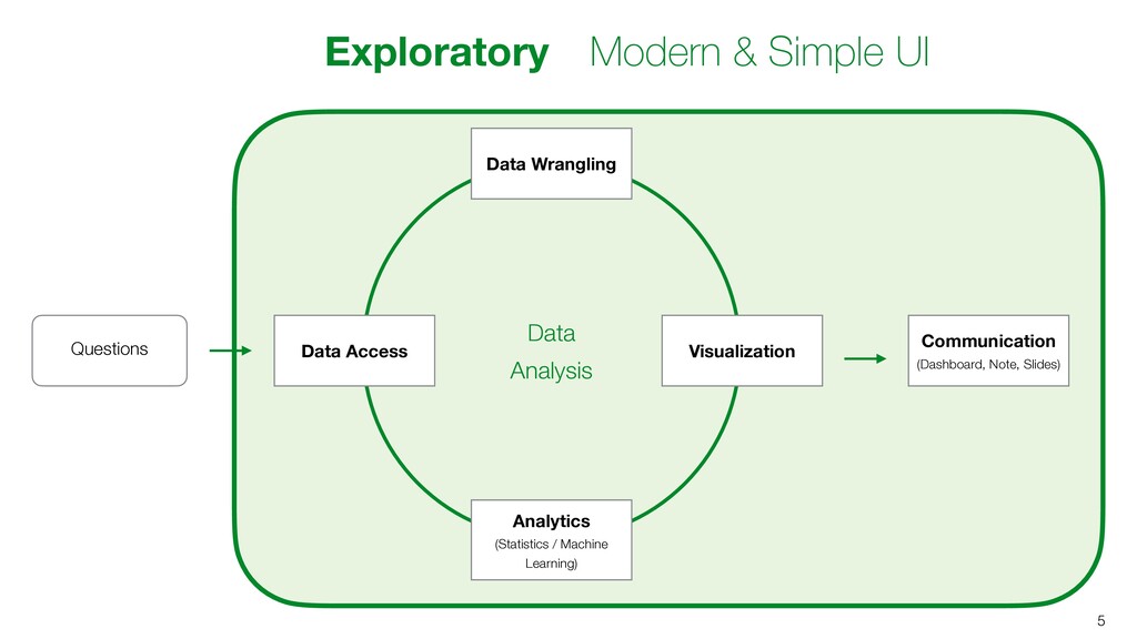
This is a part of the Exploratory Data Analysis Workshop. In this episode, we'll get into how we can find what makes a difference between two groups so that, for example, we can answer questions like "what makes a difference between those who sign up and those who don't."

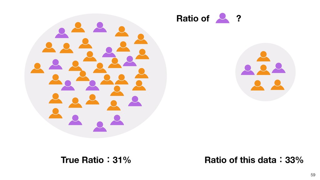
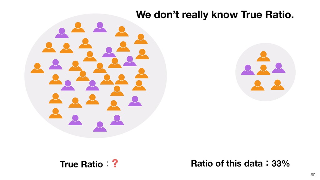
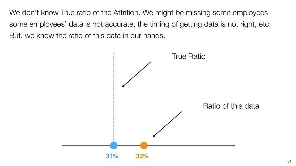
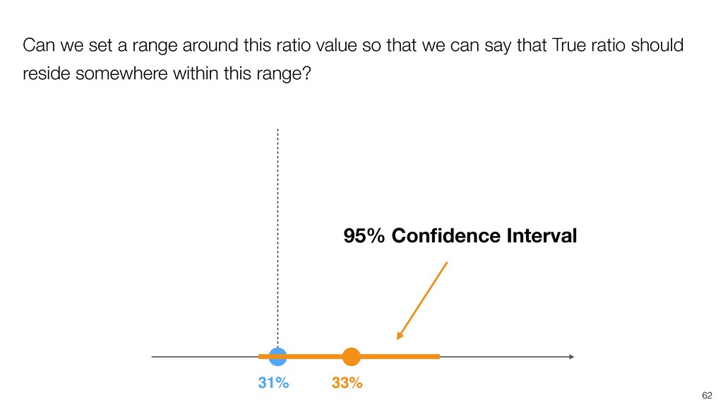
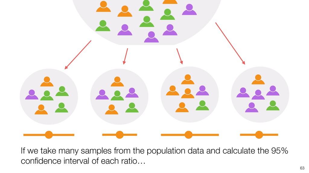
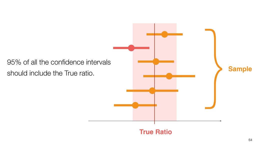
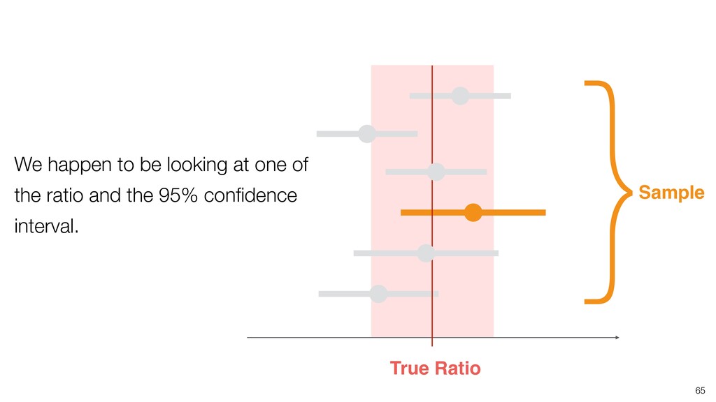
- Confidence Interval
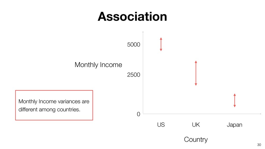
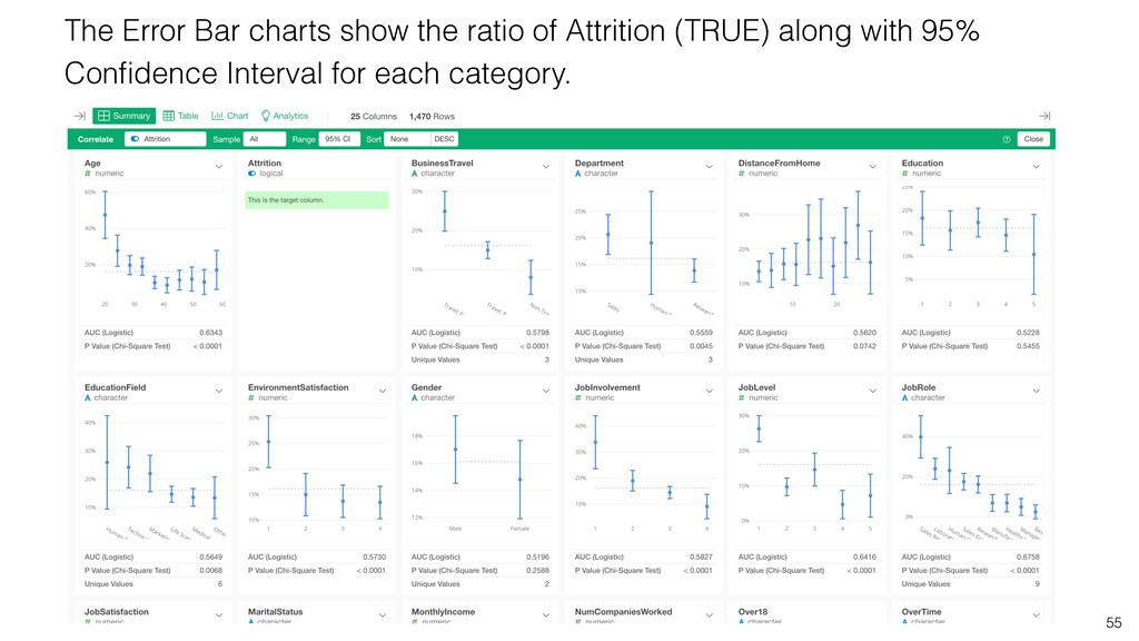
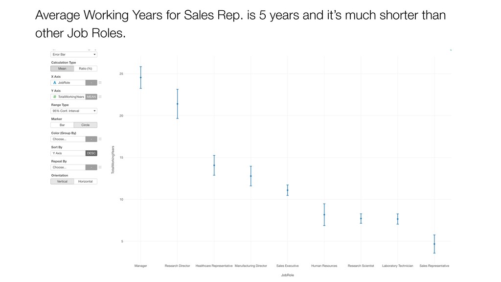
- Error Bar
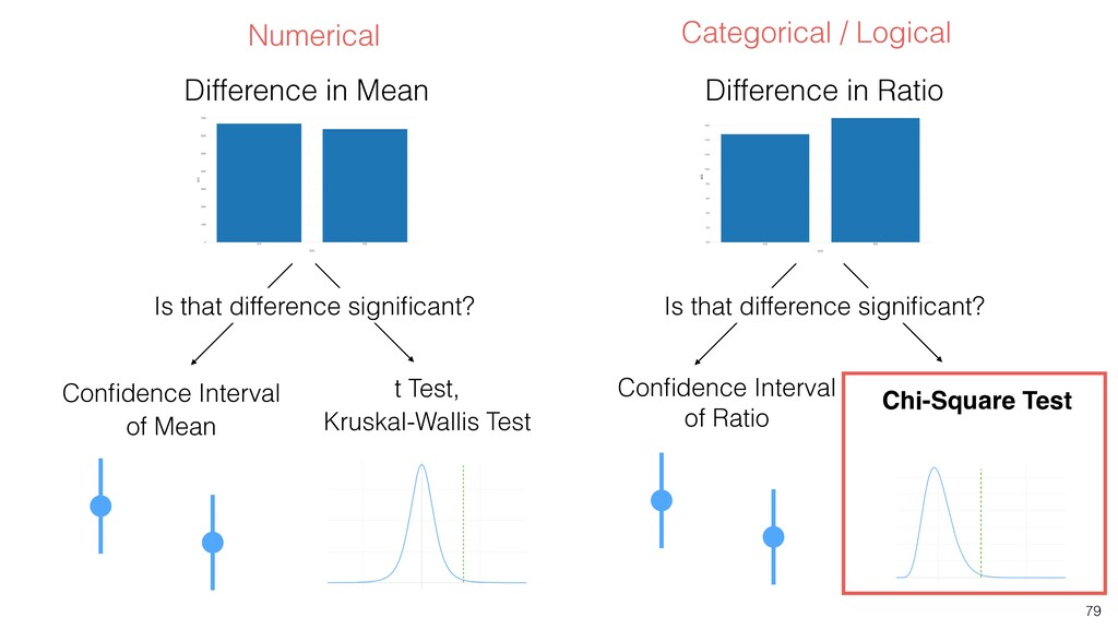
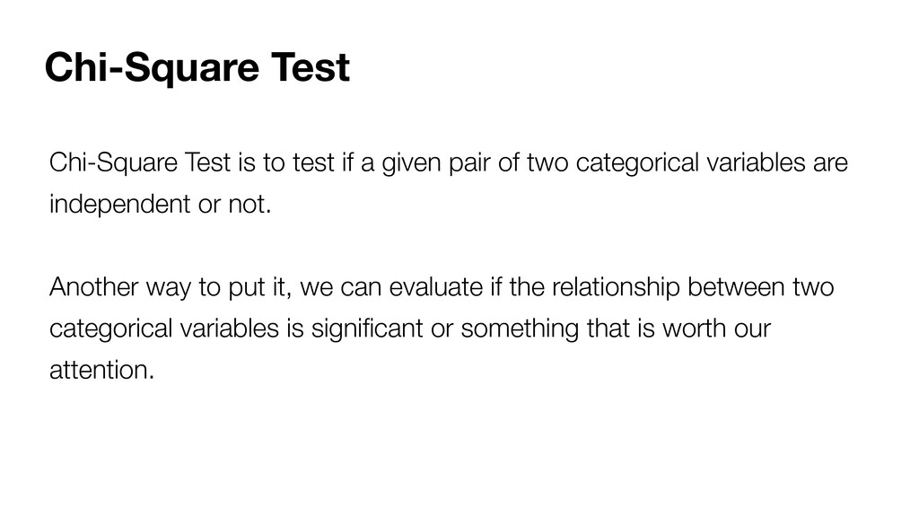
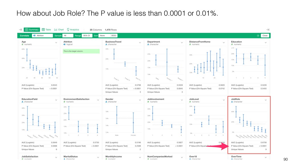
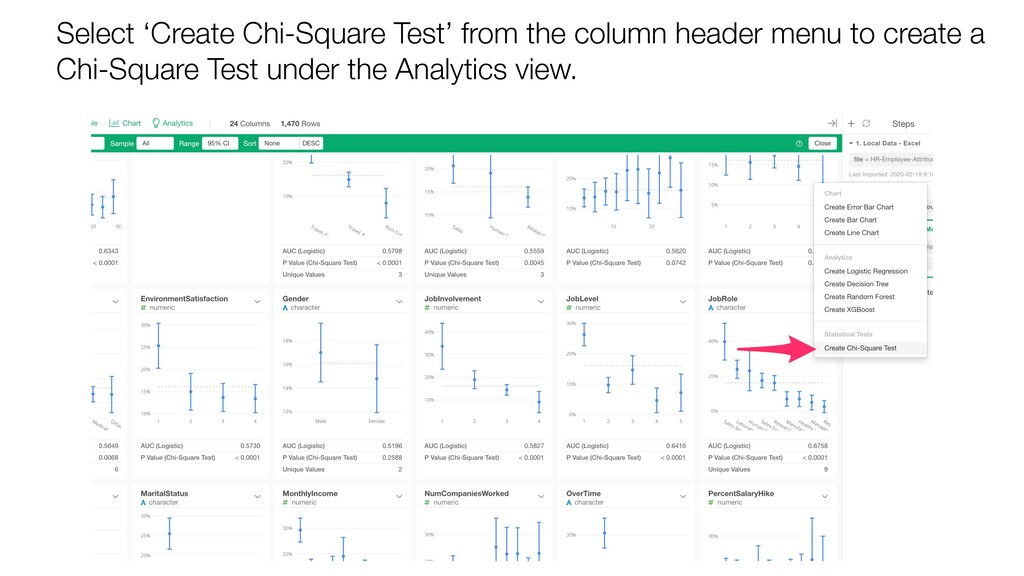
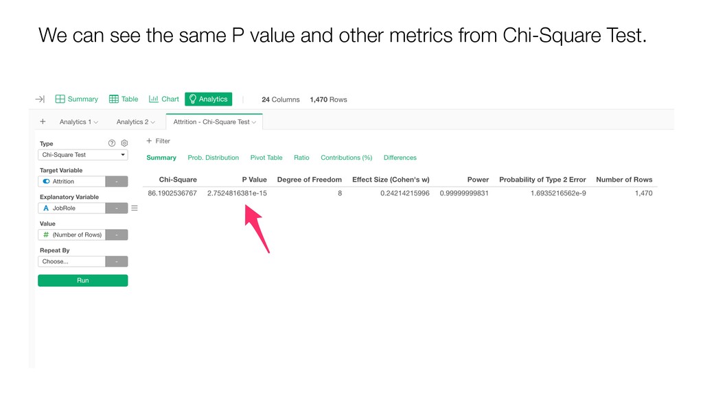
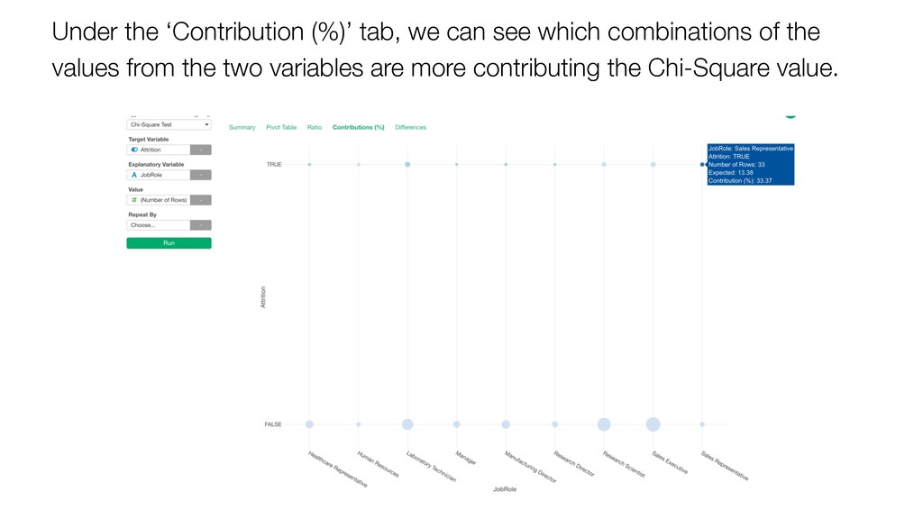
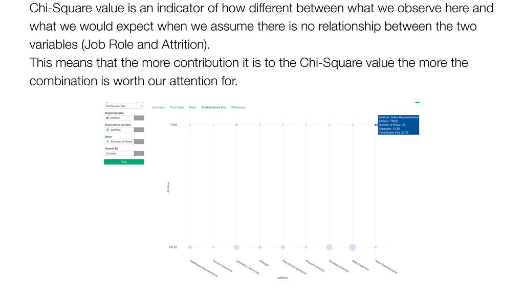
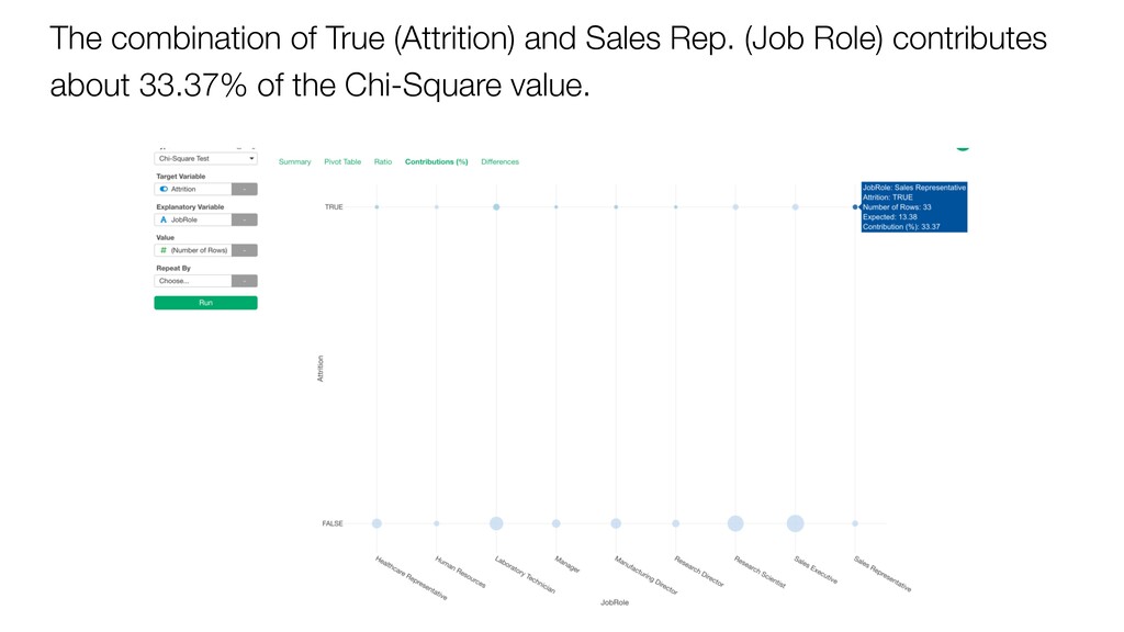
- Chi-Square Test
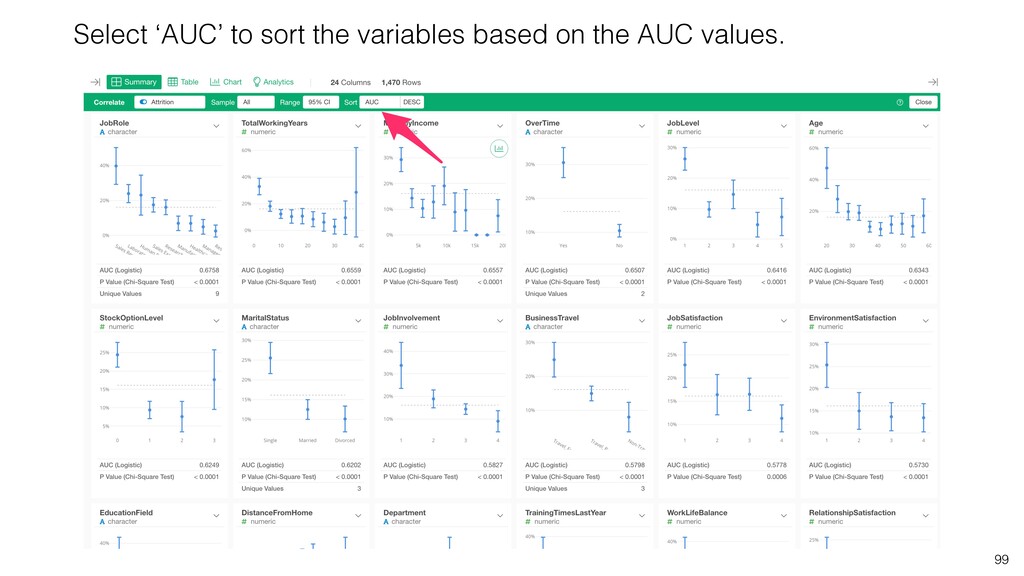
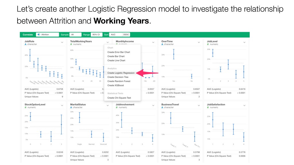
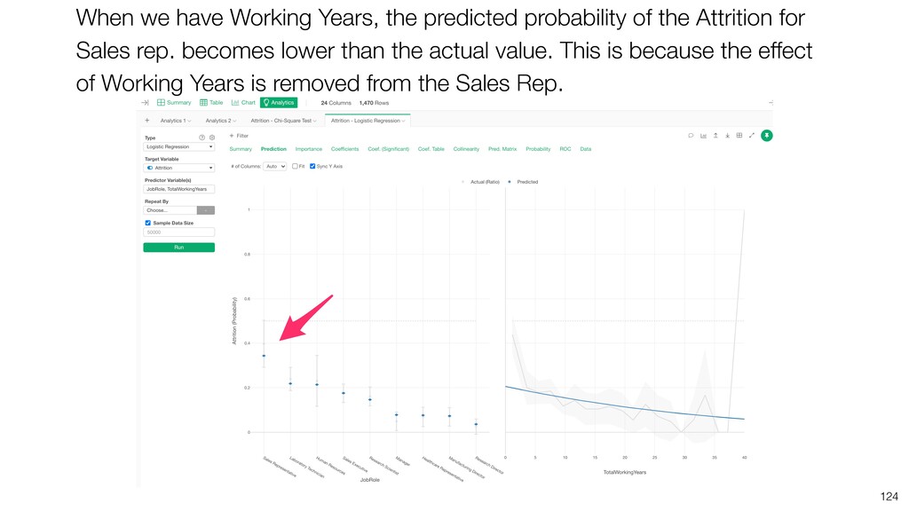
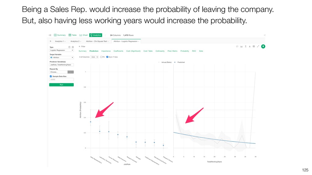
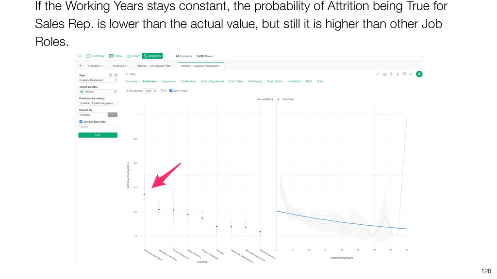
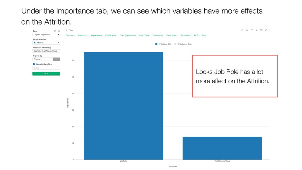
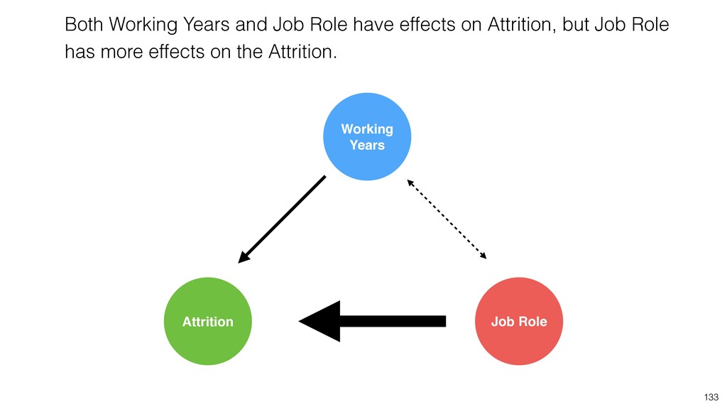
- Logistic Regression

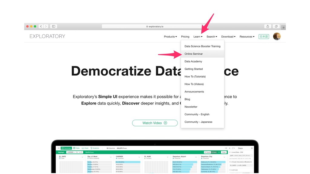
Exploratory Online Seminar: https://exploratory.io/online-seminar

The UI tool used in this video: Exploratory (https://exploratory.io)

Transcript

1. EXPLORATORY Online Seminar #33 Exploratory Data Analysis Part 3 What Makes the Difference
2. Kan Nishida CEO/co-founder Exploratory Summary In Spring 2016, launched Exploratory, Inc. to democratize Data Science. Prior to Exploratory, Kan was a director of product development at Oracle leading teams to build various Data Science products in areas including Machine Learning, BI, Data Visualization, Mobile Analytics, Big Data, etc. While at Oracle, Kan also provided training and consulting services to help organizations transform with data. @KanAugust Speaker
3. Mission Democratize Data Science
4. 4 Questions Communication Data Access Data Wrangling Visualization Analytics (Statistics / Machine Learning) Data Analysis Data Science Workflow
5. 5 Questions Communication (Dashboard, Note, Slides) Data Access Data Wrangling Visualization Analytics (Statistics / Machine Learning) Data Analysis ExploratoryɹModern & Simple UI
6. EXPLORATORY Online Seminar #33 Exploratory Data Analysis Part 3 What Makes the Difference
7. 7 Wayne Gretzky
8. 8 - Wayne Gretzky “I skate to where the puck is going to be, not where it has been.”
9. 9 Predict how many customers we will have. Prediction e.g. Customers will be 1000 by end of this year.
10. 10 - Kan Nishida “I control where the puck is going to be, not the puck controls where I should be.”
11. 11 e.g. We want to grow Customers to 1000. What can we do to make that happen? Control
12. 12 Hypothesis If the weather will be warm, we will have more customers. If we offer 10% discount, we would have more customers. Prediction Control
13. 13 Test Hypotheses by Experimenting and Collecting Data • Hypothesis Test • A/B Test Hypotheses Data Test Discount increases more customers
14. 14 Test Hypotheses by Experimenting and Collecting Data • Hypothesis Test • A/B Test Hypotheses Data Test Discount increases more customers Confirmatory Analysis
15. 15 Hypotheses Data Test How can we build Hypothesis?
16. 16 Intuition! Hypotheses Data Test
17. 17 Build Hypothesis based on Data Hypotheses Data Test Data How about Data?
18. 18 John Tukey built the method and published a book called ‘Exploratory Data Analysis’ in 1970s.
19. 19 Build hypotheses by exploring data. EDA Hypotheses Data Test Data Exploratory Data Analysis
20. An exploratory and iterative process of asking many questions and find answers from data in order to build better hypothesis for Explanation, Prediction, and Control. 20 Exploratory Data Analysis (EDA)
21. An exploratory and iterative process of asking many questions and find answers from data in order to build better hypothesis for Prediction and Control. 21 Exploratory Data Analysis (EDA)
22. 22 • How the variation in variables? • How are the variables associated (or correlated) to one another? Two Principle Questions for EDA
28. 28 A relationship where changes in one variable happen together with changes in another variable with a certain rule. Association and Correlation
29. 29 Association Correlation Any type of relationship between two variables. A certain type of (usually linear) association between two variables
30. 30 US UK Japan 5000 2500 Monthly Income variances are different among countries. Country Monthly Income 0 Association
31. 31 Age Monthly Income The bigger the Age is, the bigger the Monthly Income is. Correlation
32. 32 0 30 20 If we can find a correlation between Monthly Income and Working Years… 10 $20,000 $1,000 Working Years Monthly Income
33. 33 0 30 20 10 $20,000 $1,000 Working Years If Working Years is 20 years, Monthly Income would be around $15,000. $15,000 Monthly Income
34. 34 Income ? If we can find strong correlations, it makes it easier to explain how Monthly Income changes and to predict what Monthly Income will be.
35. Correlation is not equal to Causation. Causation is a special type of Correlation. If we can confirm a given Correlation is Causation, then we can control the outcome. Warning!
36. 36 How about the relationships between Categorical / Logical variables?
37. Employee Data
39. Categorical California Texas New York Florida Oregon
40. Categorical California Texas New York Florida Oregon No continuous relationship No ordinal relationship is necessary
42. Yes No Did this employee quit?
43. Yes No Did this employee quit? Either Yes or No Logical
44. TRUE FALSE Did this employee quit? Logical In R, there is a special data type called Logical, which can have only TRUE or FALSE. And in data analysis, we typically convert this type of columns to Logical data type.
45. TRUE FALSE YES or NO Logical Did this employee quit? 1 or 0
46. Select Change Data Type and Convert to Logical.
47. str_logical function converts a given column to Logical data type and map the values to TRUE/FALSE heuristically.
48. ‘Yes’ becomes TRUE and ‘No’ becomes ‘FALSE’. You can see the percentage of each value. It is ordered as TRUE, then FALSE.
49. 49 Attrition Country Categorical Categorical How about the relationships between Categorical / Logical variables?
50. 50 US UK Japan Country Attrition Association TRUE FALSE
51. 51 0% 20% 40% 60% 80% 100% US UK Japan Association
52. 52 Investigate how Attrition is related to other variables?
53. 53 Click on ‘Correlate’ button to open the Correlation mode.
54. 54 Select ‘Attrition’ variable (column) as the target variable.
55. 55 The Error Bar charts show the ratio of Attrition (TRUE) along with 95% Confidence Interval for each category.
56. 56 For example, we can see that employees with ‘Travel Frequently’ have higher ratio (25%) of Attrition (TRUE) compared to others.
57. For numerical variables, it divides into 10 buckets and shows the ratio and the 95% confidence interval for each bucket. 57
58. What is Confidence Interval?
59. 59 True Ratioɿ31% Ratio of this dataɿ33% Ratio of ?
60. 60 We don’t really know True Ratio. True Ratioɿ? Ratio of this dataɿ33%
61. 33% 31% True Ratio Ratio of this data 61 We don’t know True ratio of the Attrition. We might be missing some employees - some employees’ data is not accurate, the timing of getting data is not right, etc. But, we know the ratio of this data in our hands.
62. 62 Can we set a range around this ratio value so that we can say that True ratio should reside somewhere within this range? 95% Confidence Interval 33% 31%
63. 63 If we take many samples from the population data and calculate the 95% confidence interval of each ratio…
64. 64 True Ratio 95% of all the confidence intervals should include the True ratio. }Sample
65. 65 We happen to be looking at one of the ratio and the 95% confidence interval. } True Ratio Sample
66. 66 For example, we don’t know the True ratio of Attrition for ‘Travel Frequently’ but it should be somewhere between 19.82% and 30%.
67. 67 The length of the confidence interval tends to get longer when the data size is smaller, in this case, that is the number of employees. There are only 63 employees out of 1,470 in total.
68. 68 There seems to be a relationship between Attrition and Gender. It looks that Male employees tend to get higher income than Female employees.
69. 69 Attrition Gender There seems to be a relationship between Attrition and Gender. But, is that relationship really worth paying our attention?
70. 70 Numerical Variable
71. 71 Difference in Mean Numerical Income Gender
72. 72 Confidence Interval of Mean Difference in Mean Numerical Is that difference significant?
73. 73 t Test, Kruskal-Wallis Test Is that difference significant? Difference in Mean Numerical Confidence Interval of Mean
74. 2 Groups More than 2 Groups With Assumption t Test ANOVA Test No Assumption Wilcoxon Test Kruskal-Wallis Test AssumptionɿThe distribution of the original data is Normal Distribution. Various Types of Hypothesis Test 74
75. 75 Statistical Test / Hypothesis Test This significance test is based on the Kruskal-Wallis test
76. 76 Numerical Categorical Logical Target variable can be other data data type.
77. 77 Difference in Ratio Categorical / Logical Attrition Gender Is that difference significant? Difference in Mean Numerical t Test, Kruskal-Wallis Test Confidence Interval of Mean
78. 78 Confidence Interval of Ratio Is that difference significant? Difference in Mean Numerical t Test, Kruskal-Wallis Test Confidence Interval of Mean Difference in Ratio Categorical / Logical Is that difference significant?
79. Chi-Square Test 79 Is that difference significant? Difference in Mean Numerical t Test, Kruskal-Wallis Test Confidence Interval of Mean Difference in Ratio Categorical / Logical Confidence Interval of Ratio Is that difference significant?
80. Chi-Square Test is to test if a given pair of two categorical variables are independent or not. Another way to put it, we can evaluate if the relationship between two categorical variables is significant or something that is worth our attention. Chi-Square Test
81. 81 0 60 120 180 240 300 Female Male Attrition - TRUE vs. FALSE TRUE FALSE TRUE FALSE
82. 82 0% 20% 40% 60% 80% 100% Ratio TRUE FALSE TRUE FALSE Female Male
83. 83 Is this difference in the ratio between Female and Male worth our attention? Is it significant? 0% 20% 40% 60% 80% 100% TRUE FALSE TRUE FALSE Female Male
84. 84 0% 20% 40% 60% 80% 100% If there is no relationship between Attrition and Gender, then the ratio of Attrition for Female and the one for Male should be the same. Female Male
85. 85 If we assume that there is no difference between Female and Male in terms of the Attrition, the difference we are seeing with this data is big enough to be considered as ‘significant’? Or, this difference can be explained as marginal difference or just as a variance we could see with any combination of data?
86. 86 0% 20% 40% 60% 80% 100% Male 0% 20% 40% 60% 80% 100% Actual Data Theoretical Data Female Male Female Is the difference with the actual data big enough compared to the one we would expect when there is no difference?
87. 87 The P value is 0.2588, it’s about 26%.
88. It indicates the probability of observing the difference in the ratio of Attrition between Male and Female by chance when assuming that there is no relationship between Attrition and Gender variables. P Value here is 26%, which means that the chance of observing the relationship we see here is no so surprising. So the assumption above doesn’t seem to be contradicting and we can keep accepting the assumption. P-Value
89. 89 If we assume there is no difference between Attrition and Gender the chance of observing the difference we see here would be about 26%. We can conclude that there is no difference between Male and Female.
90. 90 How about Job Role? The P value is less than 0.0001 or 0.01%.
91. 91 If we assume there is no relationship between Attrition and Job Role the chance of observing the difference we see here would be close to 0%. Something that is contradicting with the assumption is happening here, so we can reject the assumption, and conclude that there is a relationship between Attrition and Job Role.
92. Chi-Square test is not just for the statistical test (hypothesis test). It can also be used to find what is something special about the relationship between two variables — Attrition and Job Role. In another word, it tells us which combinations of the values from the two variables we should pay more attention to.
93. Select ‘Create Chi-Square Test’ from the column header menu to create a Chi-Square Test under the Analytics view.
94. We can see the same P value and other metrics from Chi-Square Test.
95. Under the ‘Contribution (%)’ tab, we can see which combinations of the values from the two variables are more contributing the Chi-Square value.
96. Chi-Square value is an indicator of how different between what we observe here and what we would expect when we assume there is no relationship between the two variables (Job Role and Attrition). This means that the more contribution it is to the Chi-Square value the more the combination is worth our attention for.
97. The combination of True (Attrition) and Sales Rep. (Job Role) contributes about 33.37% of the Chi-Square value.
98. Under the Ratio tab, we can confirm that the ratio of TRUE (Attrition) in Sales Rep. is much higher than any other job types.
99. 99 Select ‘AUC’ to sort the variables based on the AUC values.
100. A metric that indicates how much a given model can separate TRUE data and FALSE data. It can be used to see the strength of the association between a given two variables. AUC (Area Under the Curve) 100 * Under the Correlation Mode, this AUC is based on a logistic regression model that is built for each variable.
101. 101 All the variables are sorted by AUC values. This means that we are seeing the variables that have stronger relationship with the Attrition variable first.a
102. Investigate the Relationship with Logistic Regression Model
103. You can create a Logistic Regression model to investigate the relationship between Attrition and Job Role further.
104. The first thing you see is a tab called ‘Prediction’ where you can see the predicted probabilities of Attrition for each Job Role.
105. It shows the probability of Attrition for each Job Role. The gray is the actual ratio of the Attrition with the 95% confidence interval. And the blue dots indicate the predicted probability of Attrition being TRUE.
106. Let’s create another Logistic Regression model to investigate the relationship between Attrition and Working Years.
107. The gray line indicates the actual ratio of the Attrition being True with the 95% confidence interval along the Working Years. And the blue line indicate the predicted probability of Attrition being TRUE.
108. You can see that the predicted probabilities of Attrition decrease as the Working Years increase.
109. 109 Both Job Role and Working Years have relationship with Attrition.
110. 110 Job Role Attrition Working Years Both Job Role and Working Years have relationship with Attrition.
111. 111 ʁ Job Role Attrition Working Years Job Role and Working Years have a relationship?
112. 112 Select Working Years as the target variable and select R-Squared to sort.
113. 113 Job Role and Working Years have a some degree of relationship.
114. 114 Relationship (Association) Job Role Attrition Working Years Job Role and Working Years have a some degree of relationship.
115. 115 Job Role Attrition Working Years Is Working Years the one having an effect on Attrition?
116. 116 Job Role Attrition Working Years Or, is Job Role the one having an effect on Attrition?
117. 117 Job Role Attrition Working Years Or, both Working Years and Job Role having an effect on Attrition?
118. 118 How can we estimate an independent (or isolated) effect for each variable? Job Role Attrition Working Years
119. 119 10 → 11 Hold constant We can allow only one of the variables to change the value while holding the other variable constant. Effect? Job Role Attrition Working Years
120. 120 Sales Rep.→ Executive 10 Job Role Attrition Working Years Hold constant Effect? We can allow only one of the variables to change the value while holding the other variable constant.
121. 121 Select Attrition as the target variable and select AUC to sort.
122. 122 Select both Job Role and Working Years, and select ‘Create Logistic Regression’ from the column header menu.
123. 123 It creates a new Logistic Regression model with 2 predictor variables of Job Role and Working Years.
124. 124 When we have Working Years, the predicted probability of the Attrition for Sales rep. becomes lower than the actual value. This is because the effect of Working Years is removed from the Sales Rep.
125. 125 Being a Sales Rep. would increase the probability of leaving the company. But, also having less working years would increase the probability.
126. Average Working Years for Sales Rep. is 5 years and it’s much shorter than other Job Roles.
127. The ratio of employees with less than 8 working years is much higher for Sales Rep. compared to other Job Roles.
128. 128 If the Working Years stays constant, the probability of Attrition being True for Sales Rep. is lower than the actual value, but still it is higher than other Job Roles.
129. 129 Same for the Working Years. When the Job Role stays constant, the slope of probability curve becomes more moderate. This is the effect of Working Years without the effect of Job Role.
130. 130 Job Role Attrition Working Years Both Working Years and Job Role have effects on Attrition.
131. Now that we know both Job Role and Working Years have some degree of relationship with Attrition. Which of the 2 variables have stronger relationship with Attrition? Or another word, Which of the 2 variables have more effect on Attrition?
132. Under the Importance tab, we can see which variables have more effects on the Attrition. Looks Job Role has a lot more effect on the Attrition.
133. 133 Job Role Attrition Working Years Both Working Years and Job Role have effects on Attrition, but Job Role has more effects on the Attrition.
134. EXPLORATORY Online Seminar #34 How to Start Exploratory for Excel Users Part 1 2/24/2021 (Wed) 11AM PT
136. Information Email kan@exploratory.io Website https://exploratory.io Twitter @ExploratoryData Seminar https://exploratory.io/online-seminar
137. Q & A 137
138. EXPLORATORY 138