DAT630 - Classification (3)

University of Stavanger, DAT630, 2016 Autumn

Transcript

1. DAT630
 Classification
 Alternative Techniques Krisztian Balog | University of Stavanger 14/09/2015 Introduction to Data Mining, Chapter 5
2. Outline - Alternative classification techniques - Rule-based - Nearest neighbors - Naive Bayes - SVM - Ensemble methods - Artificial neural networks - Class imbalance problem - Multiclass problem
3. Support Vector Machine
4. Support Vector Machine
 (SVM) - Find a linear hyperplane (decision boundary) that will separate the data
5. One possible solution B 1
6. Another possible solution B 2
7. Other possible solutions B 2
8. Which one is better? 
 B1 or B2? - How do you define better? B 1 B 2 B1 B2
9. Max. Margin Hyperplanes - Find the hyperplane that maximizes the margin B 1 B 2 b 11 b 12 b 21 b 22 margin B1 B2 margin B1
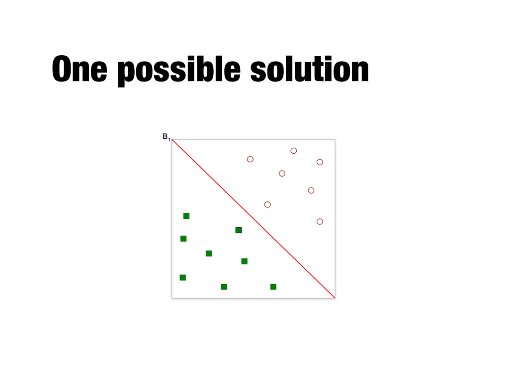
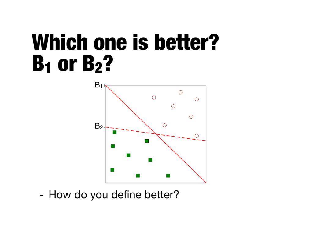
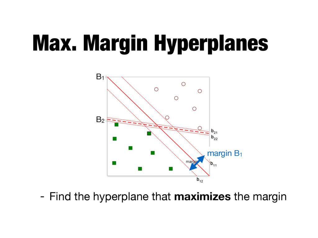
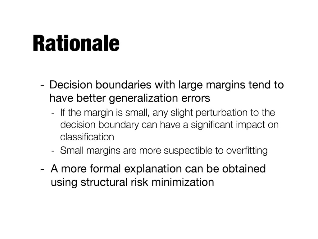
10. Rationale - Decision boundaries with large margins tend to have better generalization errors - If the margin is small, any slight perturbation to the decision boundary can have a significant impact on classification - Small margins are more suspectible to overfitting - A more formal explanation can be obtained using structural risk minimization
11. Linear SVM
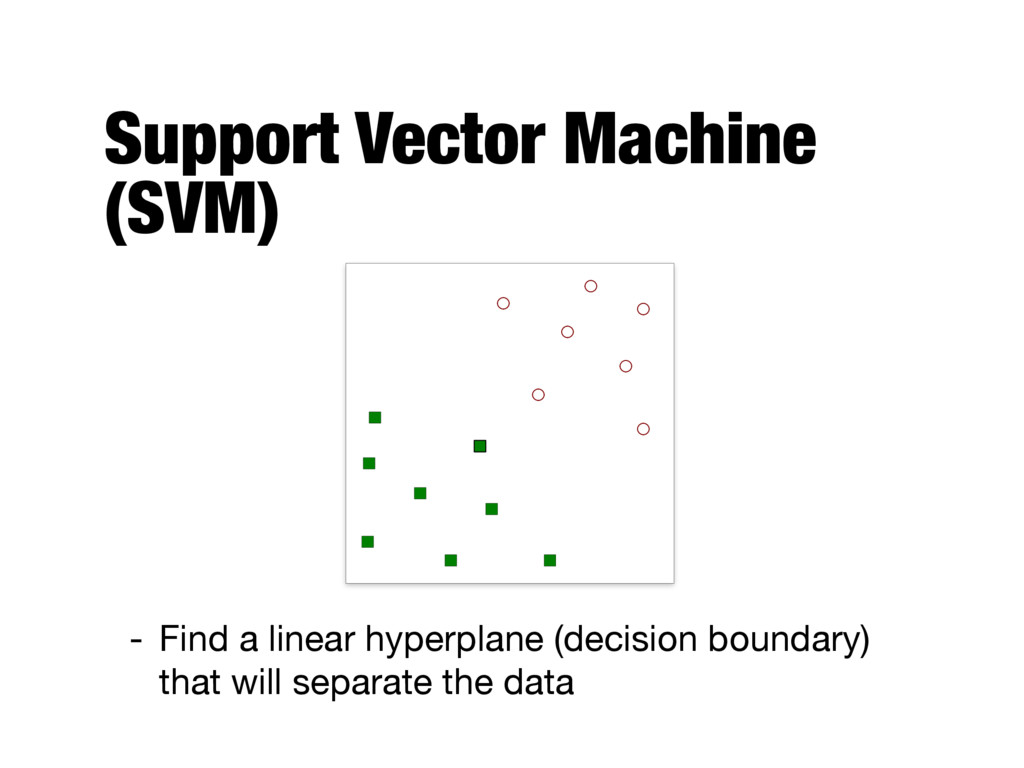
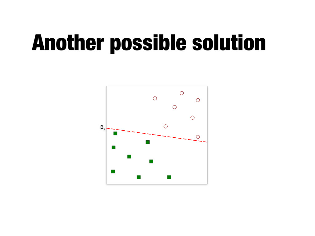
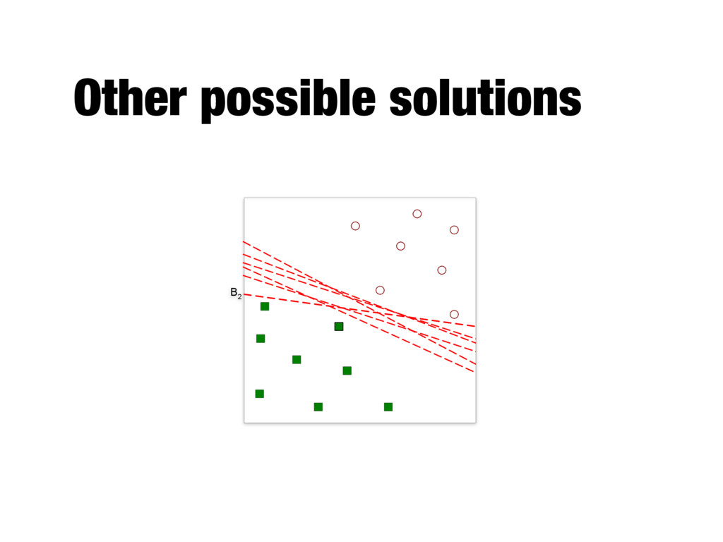
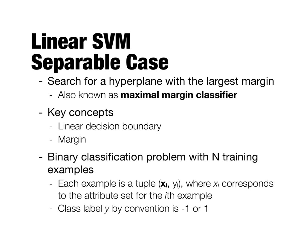
 Separable Case - Search for a hyperplane with the largest margin - Also known as maximal margin classifier - Key concepts - Linear decision boundary - Margin - Binary classification problem with N training examples - Each example is a tuple (xi, yi), where xi corresponds to the attribute set for the ith example - Class label y by convention is -1 or 1
12. Remember - Dot product of two vectors (of equal length) - Dot product of a vector with itself ~ a ·~ b = n X i=1 aibi ~ a · ~ a = ||~ a||2
13. Key Concepts B 1 b 11 b 12 Decision boundary ~ w · ~ x + b = 0 parameters of the model Hyperplanes ~ w · ~ x + b = 1 ~ w · ~ x + b = 1 Margin 2 ||~ w||2
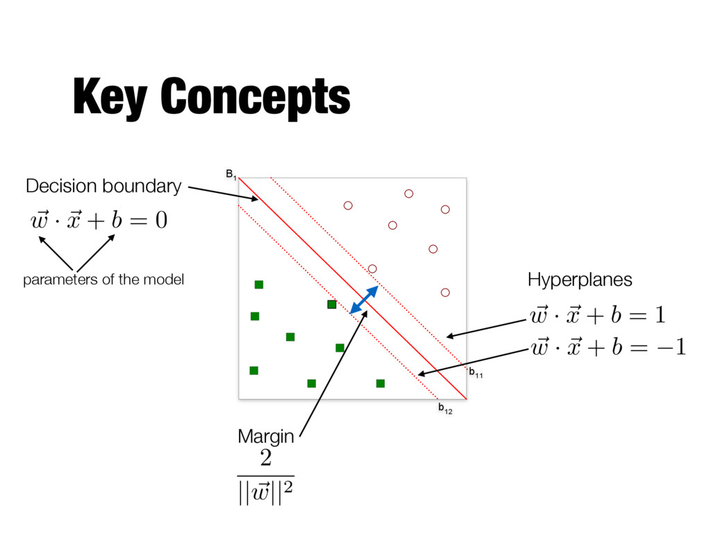
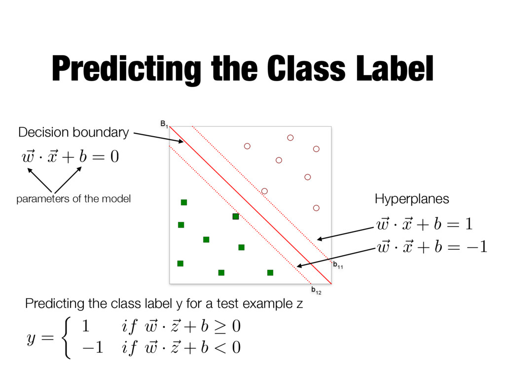
14. Predicting the Class Label B 1 b 11 b 12 Decision boundary ~ w · ~ x + b = 0 parameters of the model Hyperplanes ~ w · ~ x + b = 1 ~ w · ~ x + b = 1 Predicting the class label y for a test example z y = ⇢ 1 if ~ w · ~ z + b 0 1 if ~ w · ~ z + b < 0
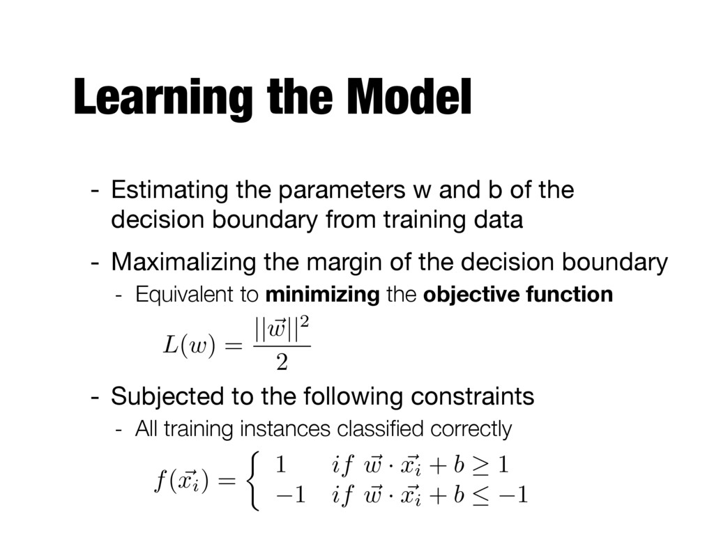
15. Learning the Model - Estimating the parameters w and b of the decision boundary from training data - Maximalizing the margin of the decision boundary - Equivalent to minimizing the objective function - Subjected to the following constraints - All training instances classified correctly L(w) = ||~ w||2 2 f ( ~ xi) = ⇢ 1 if ~ w · ~ xi + b 1 1 if ~ w · ~ xi + b  1
16. Learning the Model - Constrained optimization problem - Numerical approaches are used to solve it - Lagrange multiplier method - Karush-Kuhn-Tucker conditions - …
17. What if the problem is not linearly separable?
18. Linear SVM
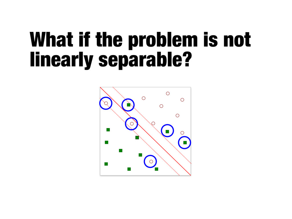
 Nonseparable Case - Learn a decision boundary that is tolerable to small training errors by using a soft margin approach - Construct a linear decision boundary even in situations where the classes are not linearly separable - Consider the trade-off between the width of the margin and the number of training errors committed by the linear decision boundary
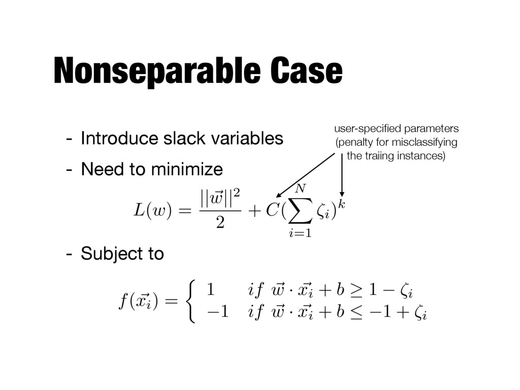
19. Nonseparable Case - Introduce slack variables - Need to minimize - Subject to L(w) = ||~ w||2 2 + C( N X i=1 ⇣i)k user-specified parameters 
 (penalty for misclassifying the traiing instances) f ( ~ xi) = ⇢ 1 if ~ w · ~ xi + b 1 ⇣i 1 if ~ w · ~ xi + b  1 + ⇣i
20. What if the decision boundary is not linear?
21. Nonlinear SVM - Trick: transform data from original coordinate space in x into a new space so that a linear decision boundary can be used ( x )
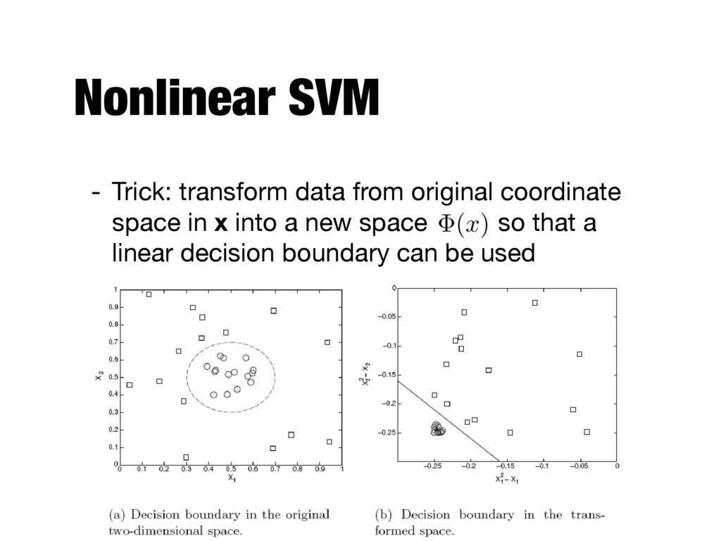
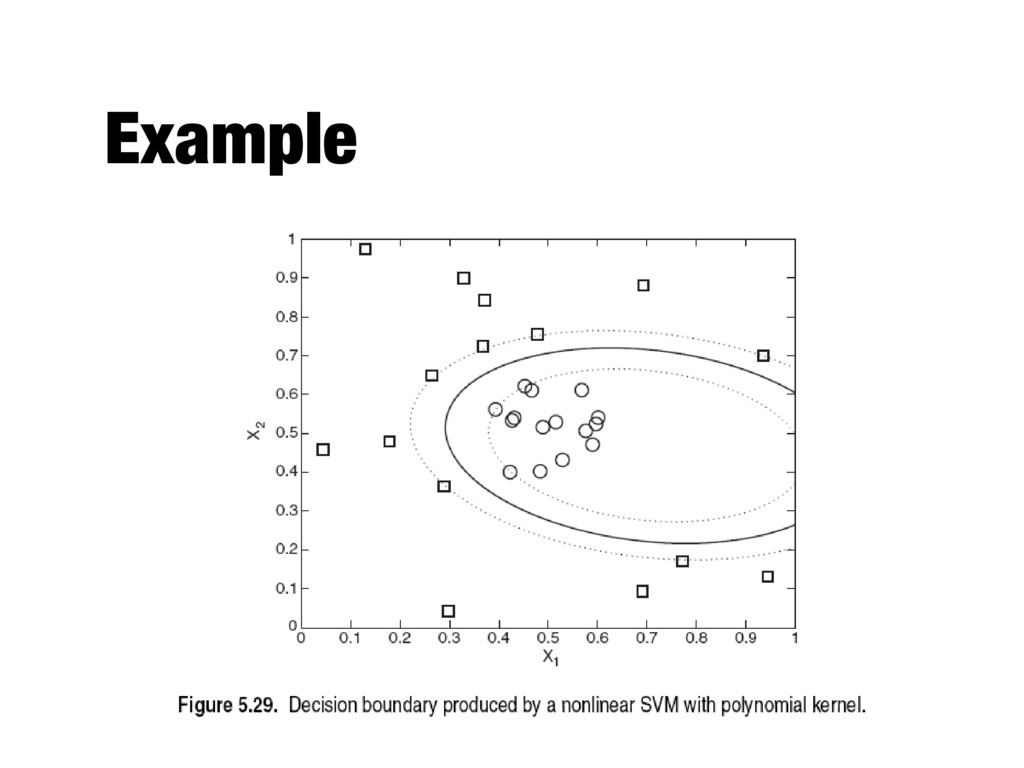
22. Problems with Transformation - Not clear what type of mapping should be used to ensure that a linear decision boundary can be constructed in the transformed space - Even if the appropriate mapping function is known, solving the constrained optimization problem in the high-dimensional feature space is computationally expensive
23. The dot product - The dot product is often regarded as a measure of similarity between two input vectors - Geometrical interpretation A · B = ||A|| ||B|| cos ✓
24. Kernel trick - The dot product can also be regarded as a measure of similarity in the transformed space - The kernel trick is a method for computing similarity in the transformed space using the original attribute set - The similarity function K which is computed in the original attribute space is known as the kernel function
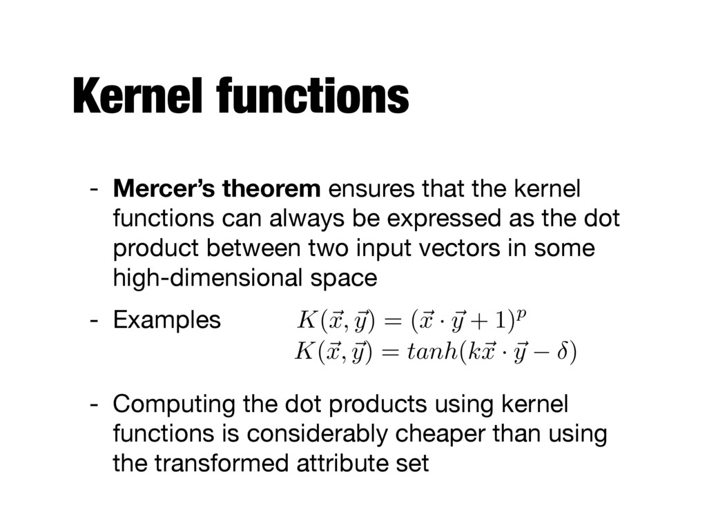
25. Kernel functions - Mercer’s theorem ensures that the kernel functions can always be expressed as the dot product between two input vectors in some high-dimensional space - Examples - Computing the dot products using kernel functions is considerably cheaper than using the transformed attribute set K ( ~ x, ~ y ) = ( ~ x · ~ y + 1)p K ( ~ x, ~ y ) = tanh ( k~ x · ~ y )
26. Example
27. Categorical attributes - SVM can be applied to categorical attributes by introducing "dummy" variables for each categorical attribute value - E.g., Martial status = {Single, Married, Divorced} - Three binary attributes: isSingle, isMarried, isDivorced
28. Summary - SVM is one of the most widely used classification algorithms - The learning problem is formulated as a convex optimization problem - Possible to find global minimum of the objective function as opposed to other classification methods - User parameters - Type of kernel function - Cost function (C) for introducing each slack variable
29. Ensemble Methods
30. Ensemble Methods - Construct a set of classifiers from the training data - Predict class label of previously unseen records by aggregating predictions made by multiple classifiers
31. General Idea
32. Random Forests
33. Artificial Neural Networks
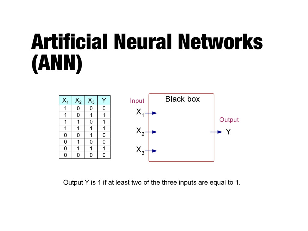
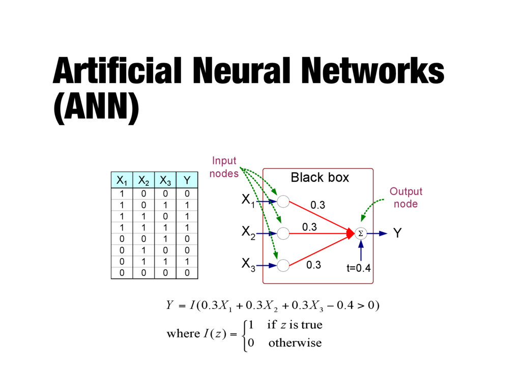
34. Artificial Neural Networks (ANN) X1 X2 X3 Y 1 0 0 0 1 0 1 1 1 1 0 1 1 1 1 1 0 0 1 0 0 1 0 0 0 1 1 1 0 0 0 0 X 1 X 2 X 3 Y Black box Output Input Output Y is 1 if at least two of the three inputs are equal to 1.
35. Artificial Neural Networks (ANN) X1 X2 X3 Y 1 0 0 0 1 0 1 1 1 1 0 1 1 1 1 1 0 0 1 0 0 1 0 0 0 1 1 1 0 0 0 0 Σ X 1 X 2 X 3 Y Black box 0.3 0.3 0.3 t=0.4 Output node Input nodes ! " # = > − + + = otherwise 0 true is if 1 ) ( where ) 0 4 . 0 3 . 0 3 . 0 3 . 0 ( 3 2 1 z z I X X X I Y
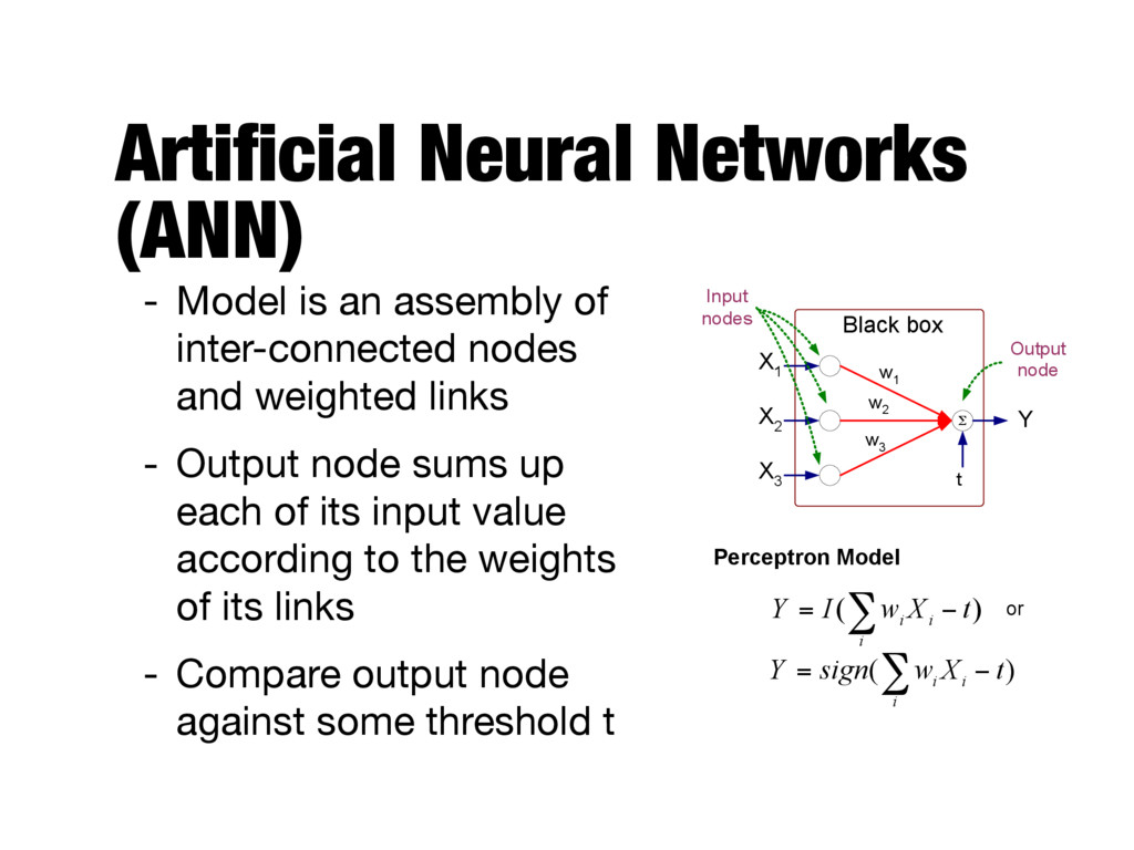
36. Artificial Neural Networks (ANN) - Model is an assembly of inter-connected nodes and weighted links - Output node sums up each of its input value according to the weights of its links - Compare output node against some threshold t Σ X 1 X 2 X 3 Y Black box w 1 t Output node Input nodes w 2 w 3 ) ( t X w I Y i i i − = ∑ Perceptron Model ) ( t X w sign Y i i i − = ∑ or
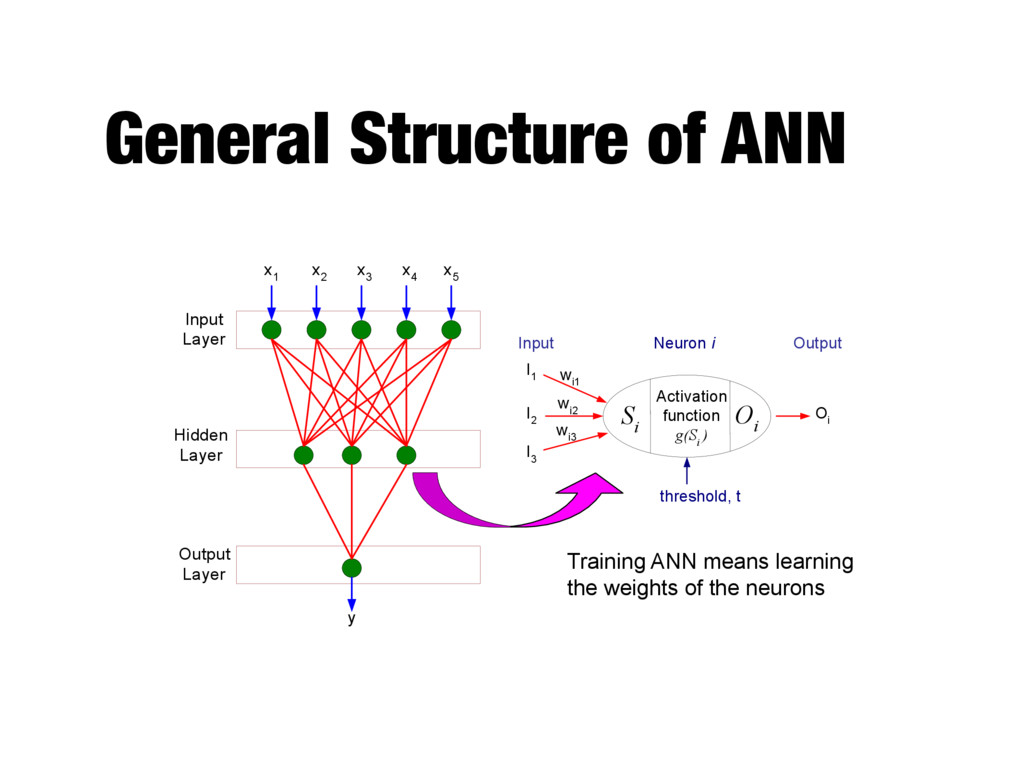
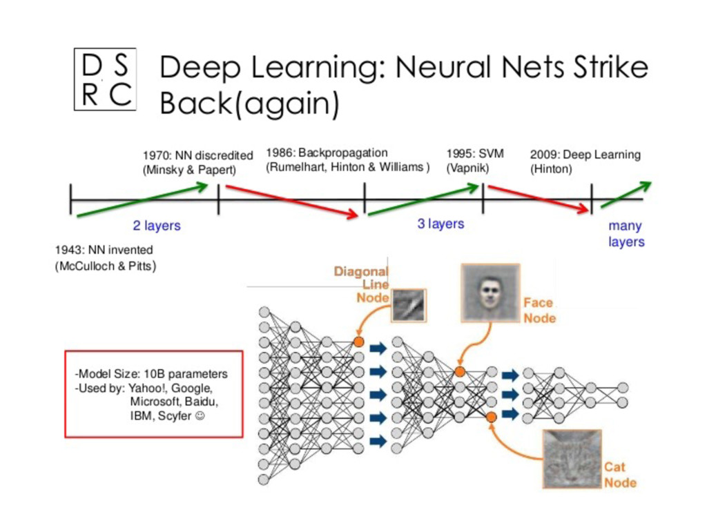
37. General Structure of ANN Activation function g(S i ) S i O i I 1 I 2 I 3 w i1 w i2 w i3 O i Neuron i Input Output threshold, t Input Layer Hidden Layer Output Layer x 1 x 2 x 3 x 4 x 5 y Training ANN means learning the weights of the neurons
38. Summary - Choosing the appropriate topology is important - Can handle redundant features well - Sensitive to the presence of noise - Training is a time consuming process
40. Class Imbalance Problem
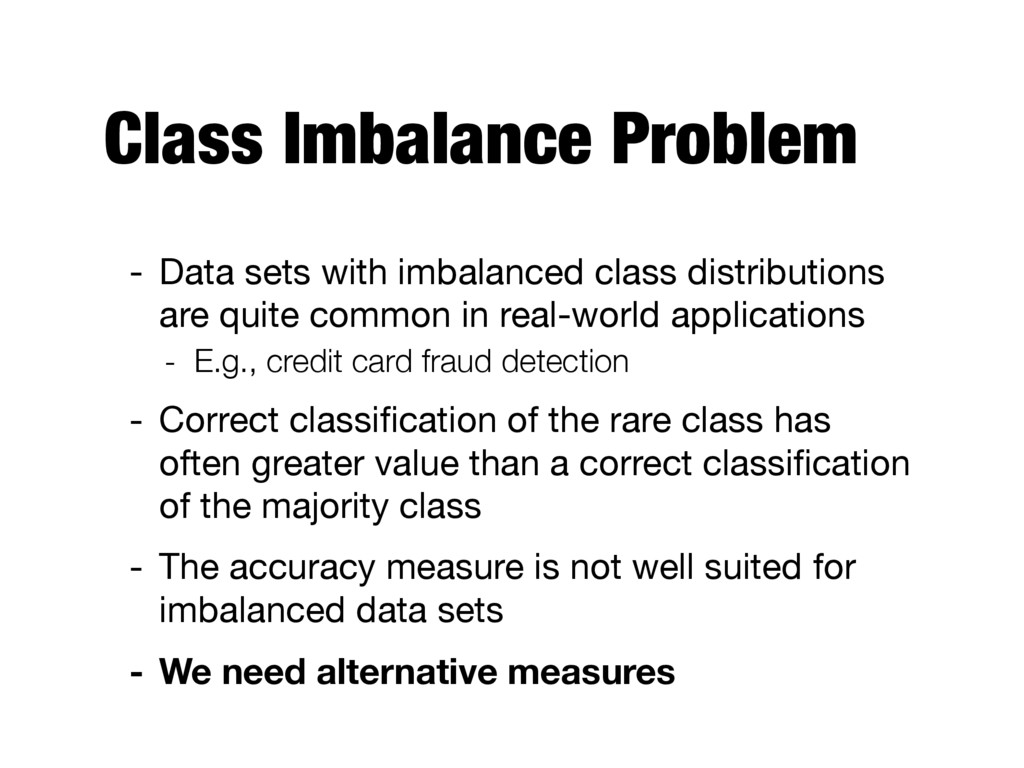
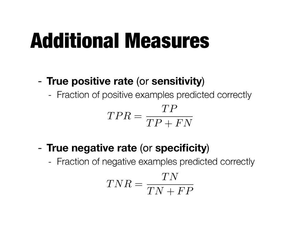
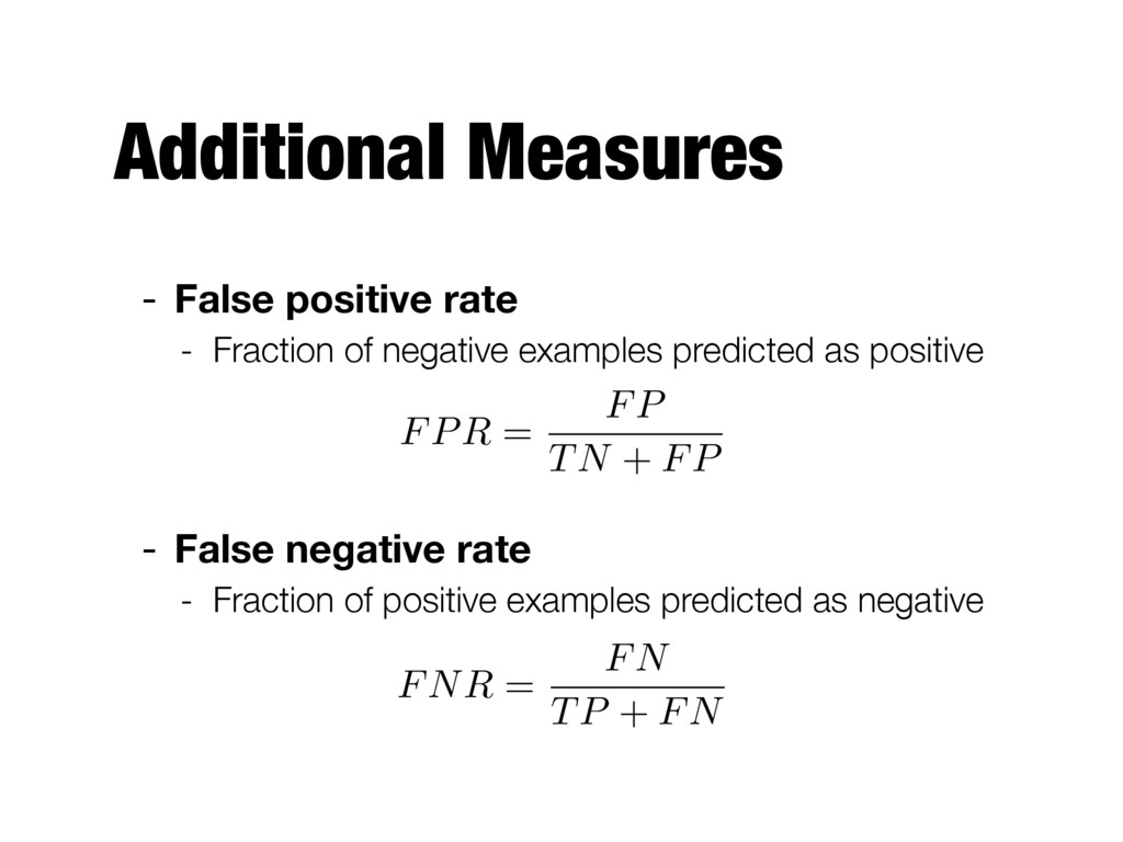
41. Class Imbalance Problem - Data sets with imbalanced class distributions are quite common in real-world applications - E.g., credit card fraud detection - Correct classification of the rare class has often greater value than a correct classification of the majority class - The accuracy measure is not well suited for imbalanced data sets - We need alternative measures
42. Confusion Matrix Predicted class Positive Negative Actual class Positive True Positives (TP) False Negatives (FN) Negative False Positives (FP) True Negatives (TN)
43. Additional Measures - True positive rate (or sensitivity) - Fraction of positive examples predicted correctly - True negative rate (or specificity) - Fraction of negative examples predicted correctly TPR = TP TP + FN TNR = TN TN + FP
44. Additional Measures - False positive rate - Fraction of negative examples predicted as positive - False negative rate - Fraction of positive examples predicted as negative FPR = FP TN + FP FNR = FN TP + FN
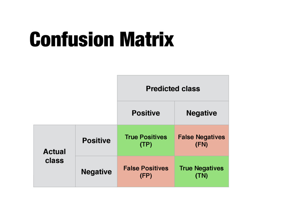
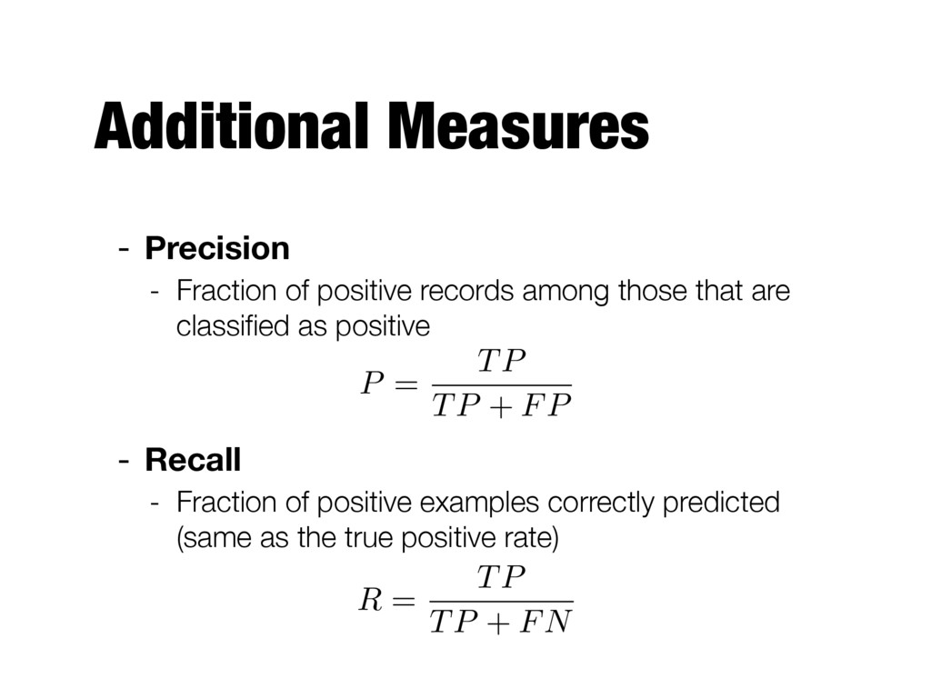
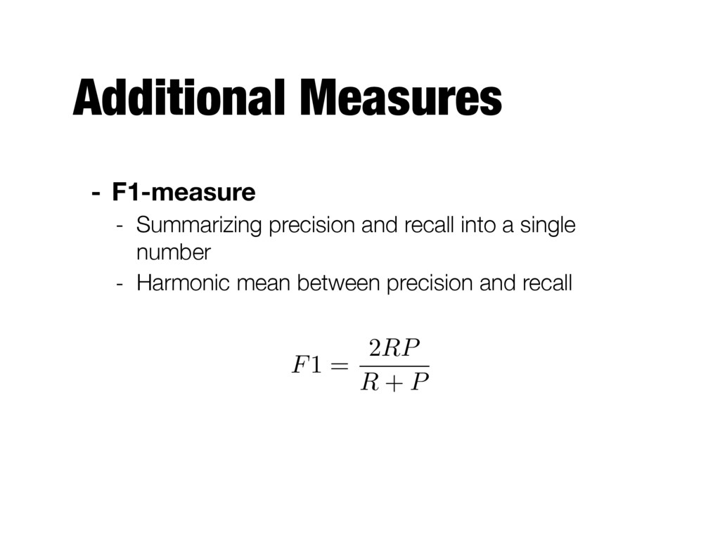
45. Additional Measures - Precision - Fraction of positive records among those that are classified as positive - Recall - Fraction of positive examples correctly predicted (same as the true positive rate) P = TP TP + FP R = TP TP + FN
46. Additional Measures - F1-measure - Summarizing precision and recall into a single number - Harmonic mean between precision and recall F1 = 2RP R + P
47. Multiclass Problem
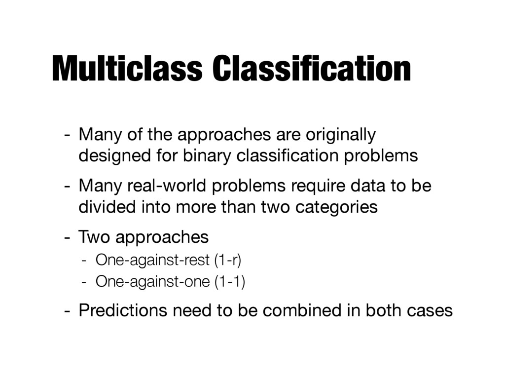
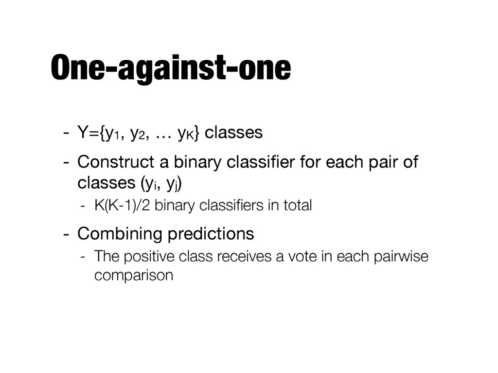
48. Multiclass Classification - Many of the approaches are originally designed for binary classification problems - Many real-world problems require data to be divided into more than two categories - Two approaches - One-against-rest (1-r) - One-against-one (1-1) - Predictions need to be combined in both cases
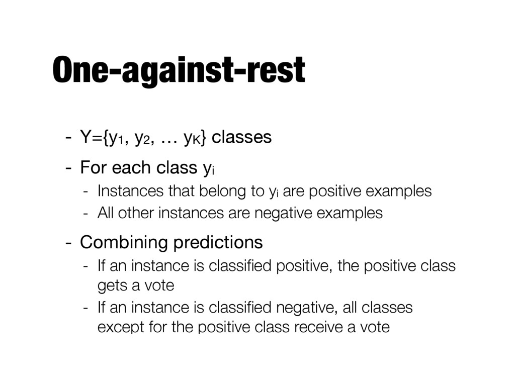
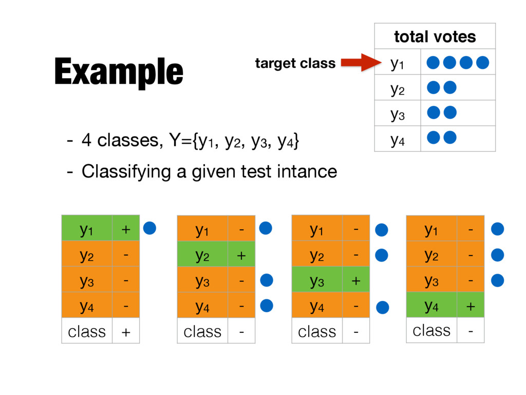
49. One-against-rest - Y={y1, y2, … yK} classes - For each class yi - Instances that belong to yi are positive examples - All other instances are negative examples - Combining predictions - If an instance is classified positive, the positive class gets a vote - If an instance is classified negative, all classes except for the positive class receive a vote
50. Example - 4 classes, Y={y1, y2, y3, y4} - Classifying a given test intance y1 + y2 - y3 - y4 - class + y1 - y2 - y3 + y4 - class - y1 - y2 + y3 - y4 - class - y1 - y2 - y3 - y4 + class - total votes y1 y2 y3 y4 target class
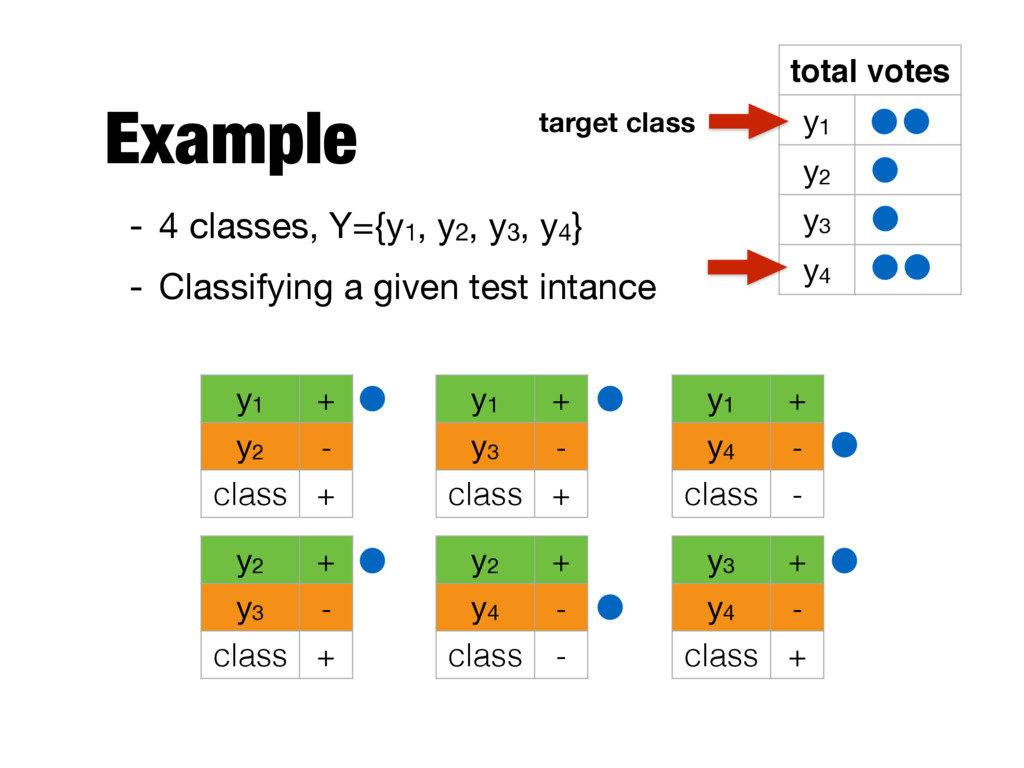
51. One-against-one - Y={y1, y2, … yK} classes - Construct a binary classifier for each pair of classes (yi, yj) - K(K-1)/2 binary classifiers in total - Combining predictions - The positive class receives a vote in each pairwise comparison
52. Example - 4 classes, Y={y1, y2, y3, y4} - Classifying a given test intance y1 + y2 - class + y1 + y3 - class + y1 + y4 - class - y2 + y3 - class + y2 + y4 - class - y3 + y4 - class + total votes y1 y2 y3 y4 target class