Accurate and efficient software microbenchmarks

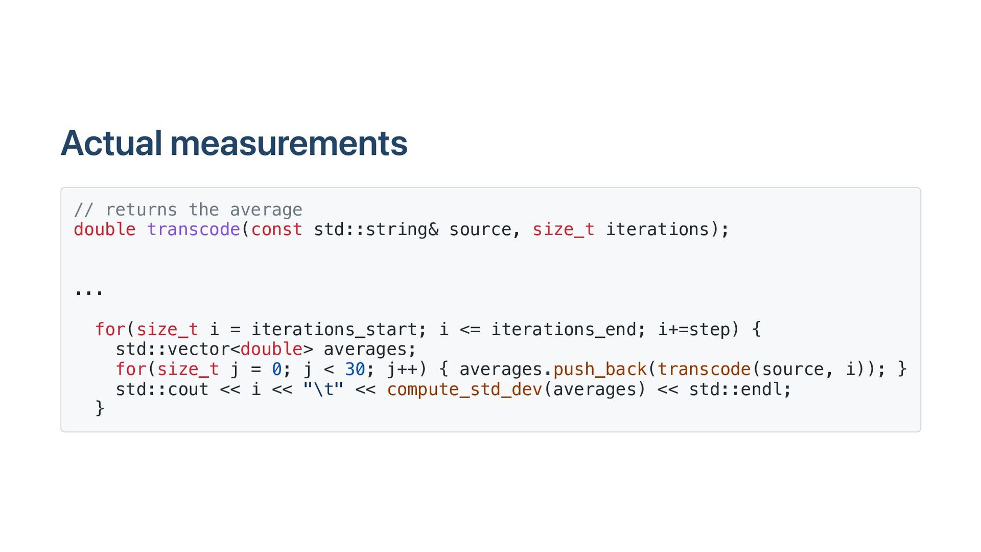
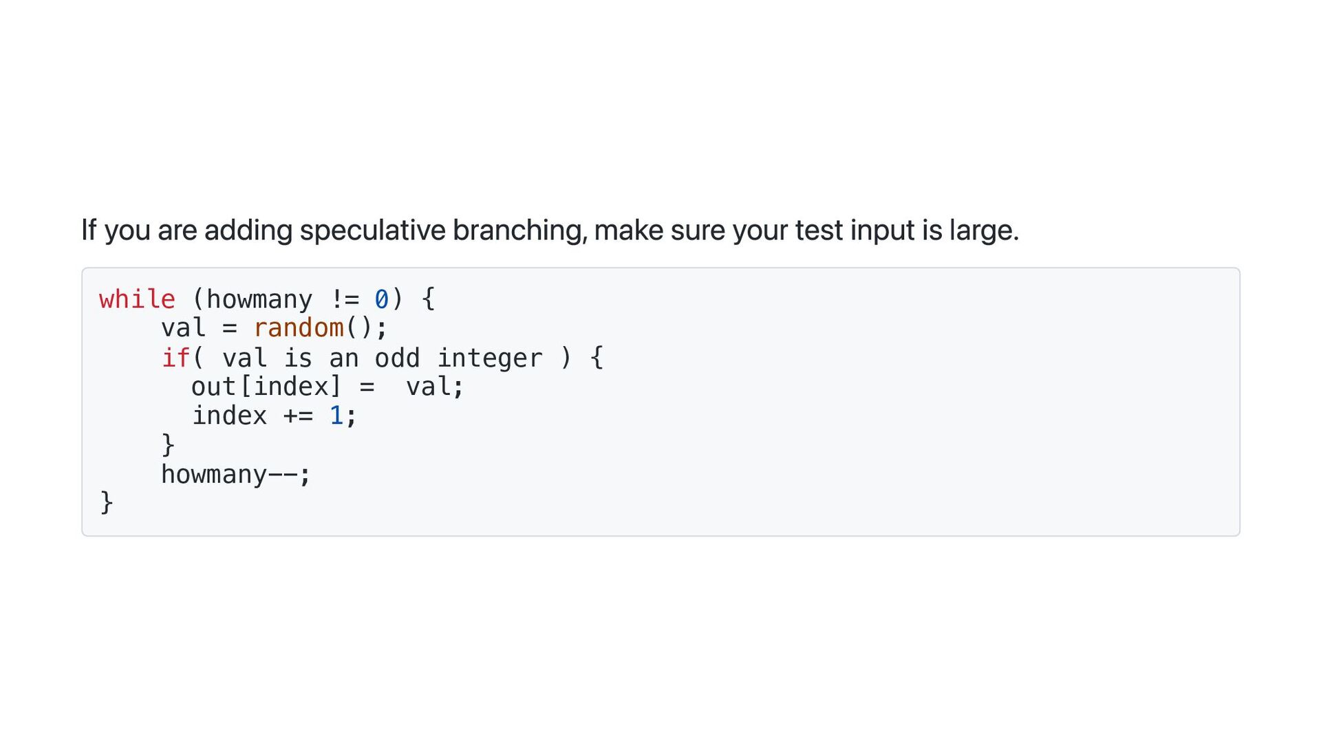
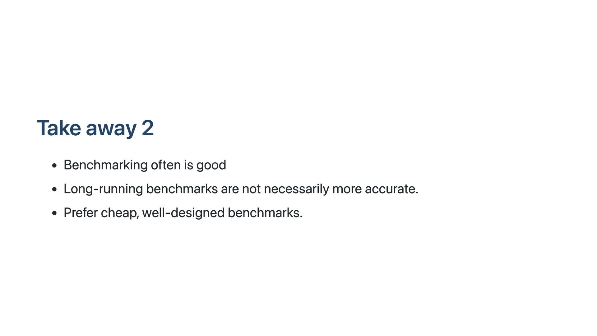
Software is often improved incrementally. Each software optimization should be assessed with microbenchmarks. In a microbenchmark, we record performance measures such as elapsed time or instruction counts during specific tasks, often in idealized conditions. In principle, the process is easy: if the new code is faster, we adopt it. Unfortunately, there are many pitfalls, such as unrealistic statistical assumptions and poorly designed benchmarks. Abstractions like cloud computing add further challenges. We illustrate effective benchmarking practices with examples.

Transcript

1. Accurate and efficient software microbenchmarks
   Daniel Lemire
   professor, Data Science Research Center
   Université du Québec (TÉLUQ)
   Montreal
   blog: https://lemire.me
   twitter: @lemire
   GitHub: https://github.com/lemire/
   

   View Slide

2. Background
   Fastest JSON parser in the world (on commodity processors):
   https://github.com/simdjson/simdjson
   First to parse JSON files at gigabytes per second
   

   View Slide

3. Where is the code ?
   All code for this talk is online (reproducible!!!)
   https://github.com/lemire/talks/tree/master/2023/performance/code
   

   View Slide

4. How fast is your disk?
   PCIe 4 drives: 5 GB/s reading speed (sequential)
   PCIe 5 drives: 10 GB/s reading speed (sequential)
   

   View Slide

5. CPU Frequencies are stagnating
   architecture availability max. frequency
   Intel Skylake 2015 4.5 GHz
   Intel Ice Lake 2019 4.1 GHz
   

   View Slide

6. Fact
   Single-core processes are often CPU bound
   

   View Slide

7. Solution?
   Optimize the software.
   Incremental optimization, how do you know that you are on the right track?
   

   View Slide

8. Hypothesis
   This software change (commit) improves our performance.
   

   View Slide

9. Simple
   Measure time elapsed before, time elapsed after.
   

   View Slide

10. Complex system
    Software systems are complex systems: changes can have unexpected consequences.
    

    View Slide

11. JIT
    Virtual Machine Warmup Blows Hot and Cold
    

    View Slide

12. System calls
    System calls (especially IO) may dominate, assume that they remain constant. Idem with
    multicore and multi-system processes.
    

    View Slide

13. Data access
    data structure layout changes can trigger expensive loads, assume that we keep that
    constant.
    

    View Slide

14. Tiny functions
    Uncertainty principle: by measuring you are affecting the execution so that you cannot
    measure safely tiny functions.
    

    View Slide

15. Take statically compiled code
    Transcoding UTF-16 to UTF-8 of an 80kB Arabic string using the simdutf library (NEON
    kernel).
    

    View Slide

16. Use the average?
    Let be the true value and let be the noise distribution (variance ).
    We seek .
    

    View Slide

17. Repeated measures increase accuracy
    Measures are
    Sum is . Variance is .
    Average is . Variance is . Standard deviation of .
    

    View Slide

18. Simulation
    mu, sigma = 10000, 5000
    for N in range(20, 2000+1):
    s = [sum(np.random.default_rng().normal(mu, sigma, N))/N for i in range(30)]
    print(N,np.std(s))
    

    View Slide

19. View Slide

20. Actual measurements
    // returns the average
    double transcode(const std::string& source, size_t iterations);
    ...
    for(size_t i = iterations_start; i <= iterations_end; i+=step) {
    std::vector averages;
    for(size_t j = 0; j < 30; j++) { averages.push_back(transcode(source, i)); }
    std::cout << i << "\t" << compute_std_dev(averages) << std::endl;
    }
    

    View Slide

21. View Slide

22. Sigma events
    

    View Slide

23. 1-sigma is 32%
    2-sigma is 5%
    3-sigma is 0.3% (once ever 300 trials)
    4-sigma is 0.00669% (once every 15000 trials)
    5-sigma is 5.9e-05% (once every 1,700,000 trials)
    6-sigma is 2e-07% (once every 500,000,000)
    for
    

    View Slide

24. Measuring sigma events
    Take 300 measures after warmup, and measure the worst relative deviation
    $ for i in {1..10}; do sudo ./sigma_test; done
    4.56151
    4.904
    7.43446
    5.73425
    9.89544
    12.975
    3.92584
    3.14633
    4.91766
    5.3699
    

    View Slide

25. What if we dealt with log-normal distributions?
    

    View Slide

26. for N in range(20, 2000+1):
    s = [sum(np.random.default_rng().lognormal(1, 4, N))/N for i in range(30)]
    print(N,np.std(s))
    

    View Slide

27. View Slide

28. What if we measured the minimum?
    Relative standard deviation ( )
    N average minimum
    200 3.44% 1.38%
    2000 2.66% 1.19%
    10000 2.95% 1.27%
    

    View Slide

29. The minimum is easier to measure to 1% accuracy.
    

    View Slide

30. CPU performance counters
    Processors have zero-overhead counters recording instruction retired, actual cycles, and
    so forth.
    No need to freeze the CPU frequency: you can measure it.
    

    View Slide

31. Limitations
    You can only measure so many things (2, 4 metrics, not 25)
    Required privileged access (e.g., root)
    

    View Slide

32. Counters in the cloud
    x64: Requires at least a full CPU
    ARM Graviton: generally available but limited number (e.g., 2 counters)
    

    View Slide

33. Instruction counts are accurate
    

    View Slide

34. Using performance counters
    Java instruction counters: https://github.com/jvm-profiling-tools/async-profiler
    C/C++: instruction counters are available through the Linux kernel
    Go instruction counters
    

    View Slide

35. Generally, fewer instructions means faster code
    Some instructions are more expensive than others (e.g., division).
    Data dependency can make instruction counts less relevant.
    Branching can artificially lower instruction count.
    

    View Slide

36. If you are adding speculative branching, make sure your test input is large.
    while (howmany != 0) {
    val = random();
    if( val is an odd integer ) {
    out[index] = val;
    index += 1;
    }
    howmany--;
    }
    

    View Slide

37. 2000 'random' elements, AMD Rome
    trial mispredicted branches
    1 50%
    2 18%
    3 6%
    4 2%
    5 1%
    6 0.3%
    7 0.15%
    8 0.15%
    

    View Slide

38. Take away 1
    Computational microbenchmarks can have log-normal distributions.
    Consider measuring the minimum instead of the average.
    

    View Slide

39. Take away 2
    Benchmarking often is good
    Long-running benchmarks are not necessarily more accurate.
    Prefer cheap, well-designed benchmarks.
    

    View Slide

40. Links
    Blog https://lemire.me/blog/
    Twitter: @lemire
    GitHub: https://github.com/lemire
    

    View Slide