ICIP 2015 - Multivalued label diffusion

Transcript

1. Multivalued Label Diffusion for Semi-supervised Segmentation Multivalued Label Diffusion for Semi-supervised Segmentation Pierre Buyssens, Olivier Lézoray GREYC UMR CNRS 6072, Image Team, University of Caen 28/09/2015 1/32
2. Multivalued Label Diffusion for Semi-supervised Segmentation Previous work 1 Previous work Region growing diffusion Example of application : Superpixels Limitations 2 Proposed method Principle Results & Comparisons Texture segmentation 2/32
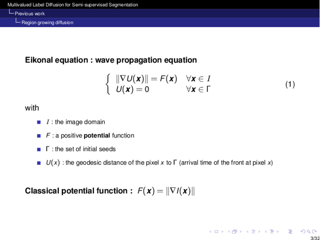
3. Multivalued Label Diffusion for Semi-supervised Segmentation Previous work Region growing diffusion Eikonal equation : wave propagation equation ⇢ k— U ( x )k = F ( x ) 8 x 2 I U ( x ) = 0 8 x 2 (1) with I : the image domain F : a positive potential function : the set of initial seeds U ( x ) : the geodesic distance of the pixel x to (arrival time of the front at pixel x ) Classical potential function : F ( x ) = k— I ( x )k 3/32
4. Multivalued Label Diffusion for Semi-supervised Segmentation Previous work Region growing diffusion 4/32
5. Multivalued Label Diffusion for Semi-supervised Segmentation Previous work Region growing diffusion 5/32
6. Multivalued Label Diffusion for Semi-supervised Segmentation Previous work Region growing diffusion 6/32
7. Multivalued Label Diffusion for Semi-supervised Segmentation Previous work Region growing diffusion 7/32
8. Multivalued Label Diffusion for Semi-supervised Segmentation Previous work Region growing diffusion 8/32
9. Multivalued Label Diffusion for Semi-supervised Segmentation Previous work Region growing diffusion 9/32
10. Multivalued Label Diffusion for Semi-supervised Segmentation Previous work Region growing diffusion 10/32
11. Multivalued Label Diffusion for Semi-supervised Segmentation Previous work Region growing diffusion 11/32
12. Multivalued Label Diffusion for Semi-supervised Segmentation Previous work Region growing diffusion 12/32
13. Multivalued Label Diffusion for Semi-supervised Segmentation Previous work Region growing diffusion 13/32
14. Multivalued Label Diffusion for Semi-supervised Segmentation Previous work Region growing diffusion 14/32
15. Multivalued Label Diffusion for Semi-supervised Segmentation Previous work Region growing diffusion 15/32
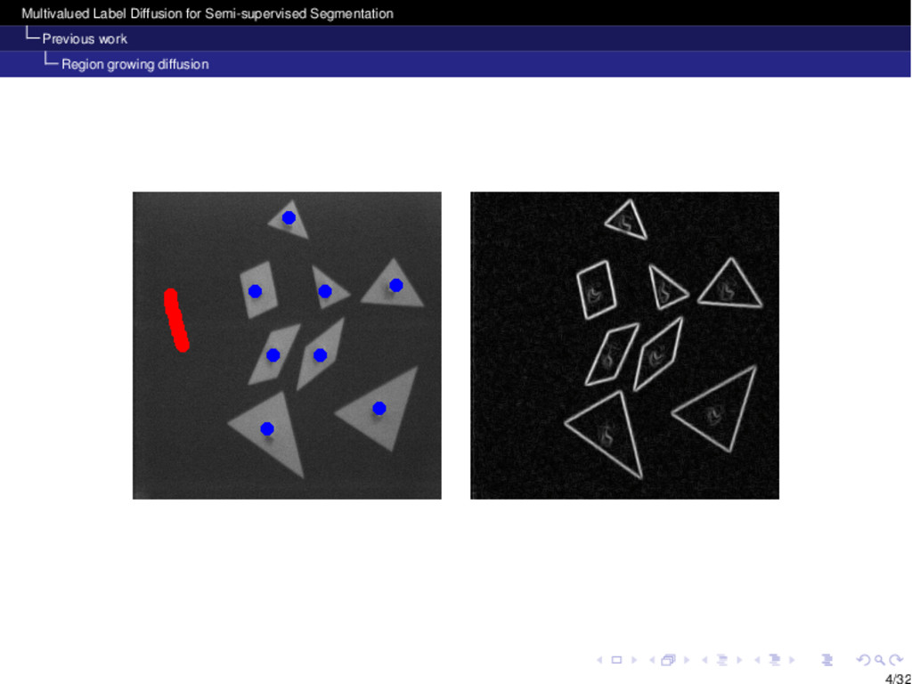
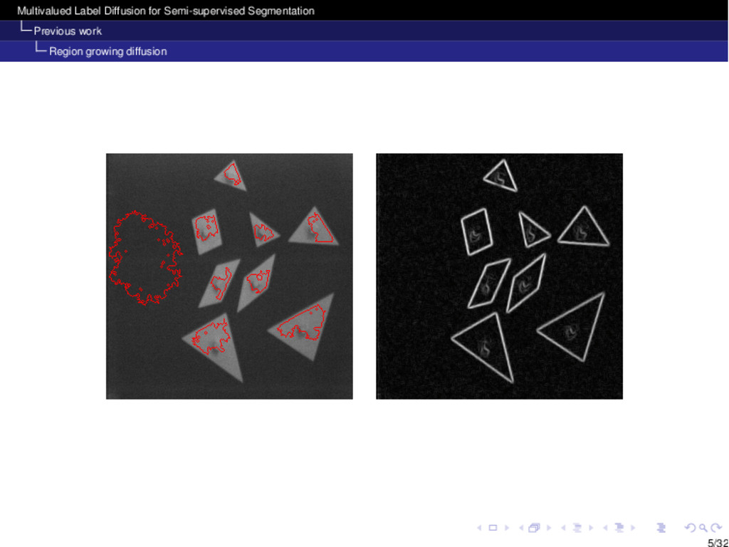
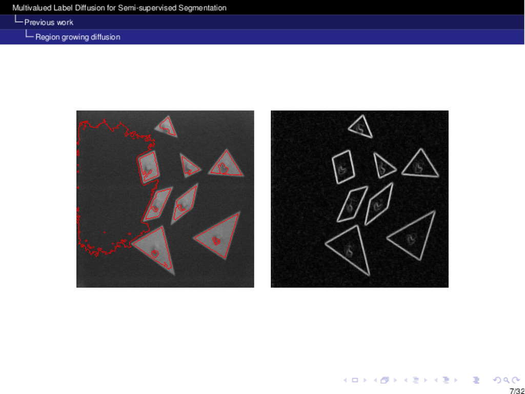
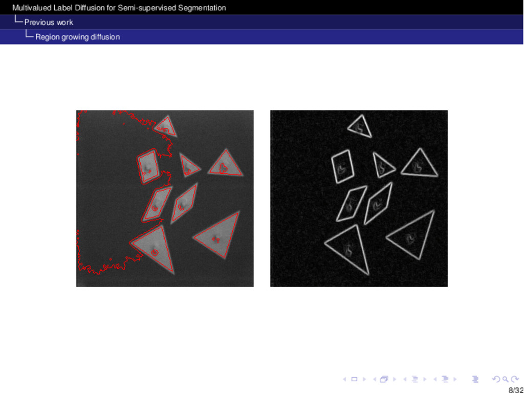
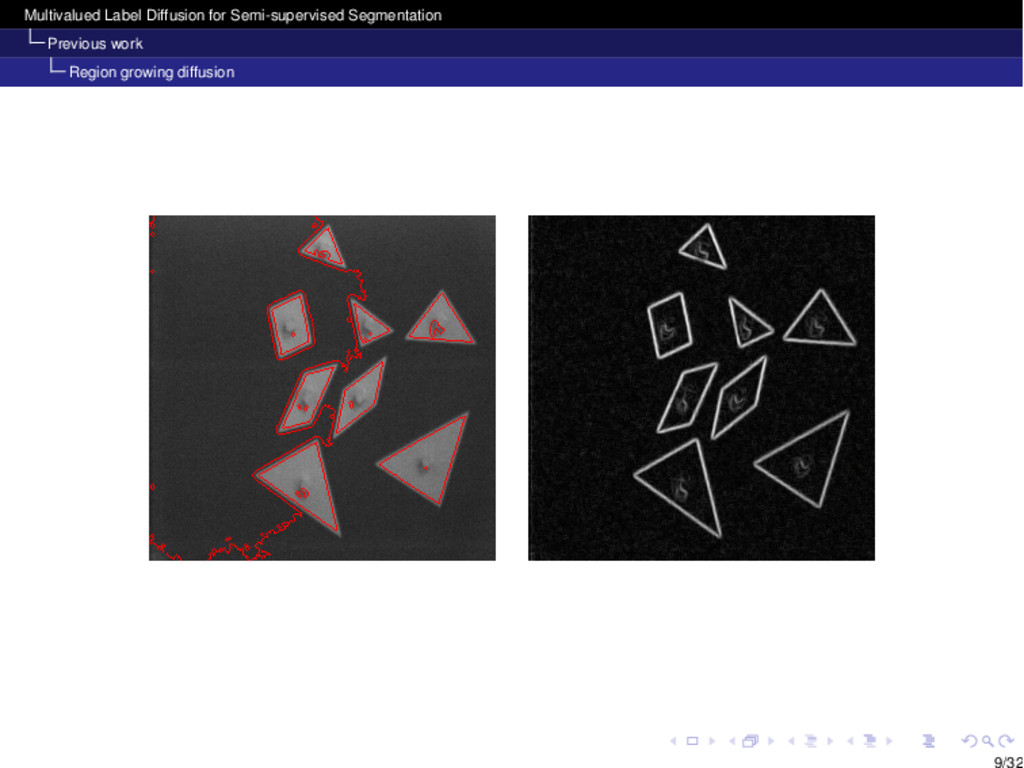
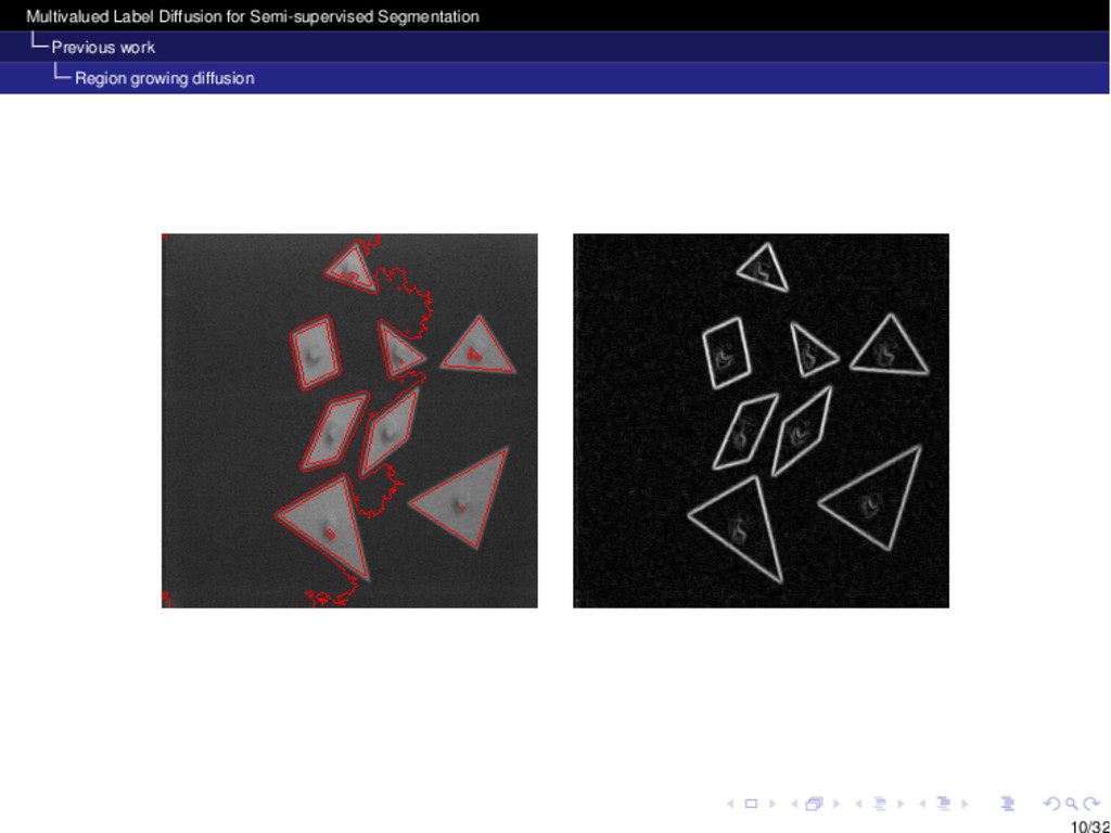
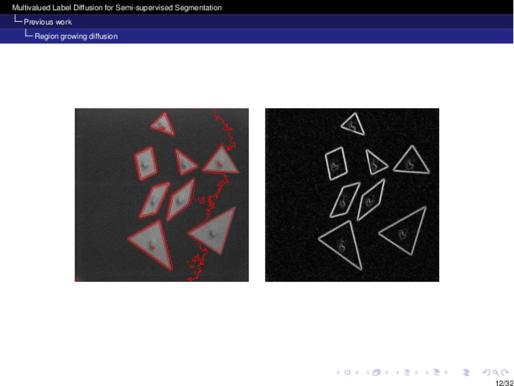
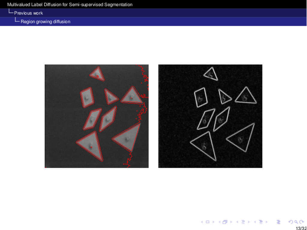
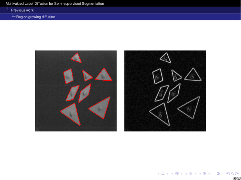
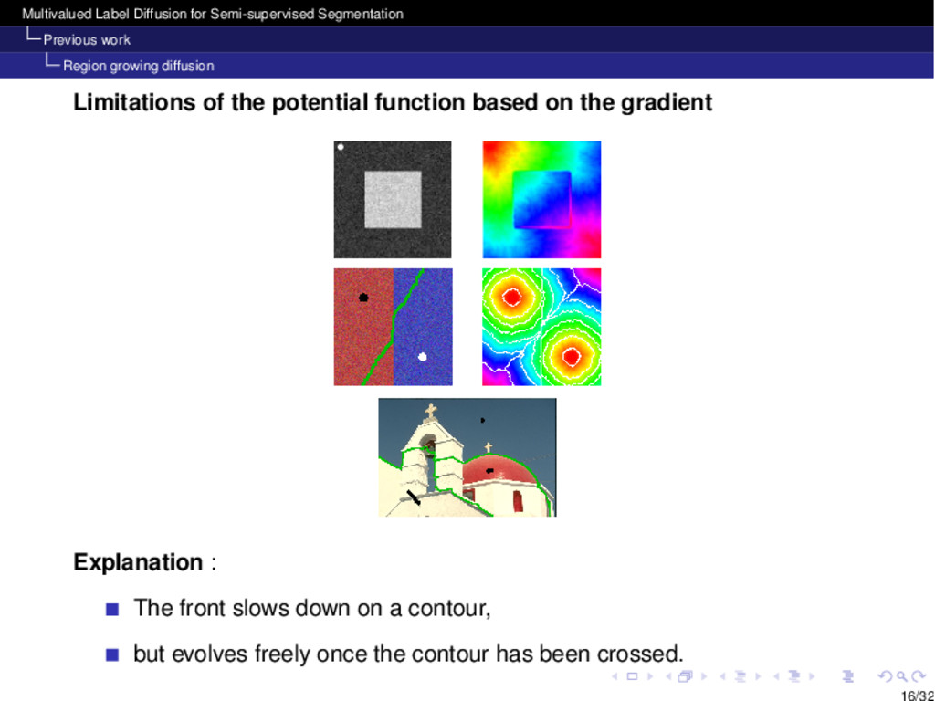
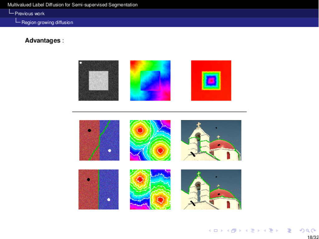
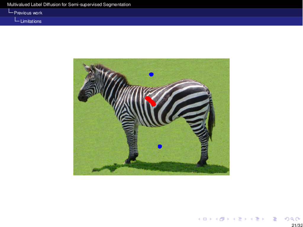
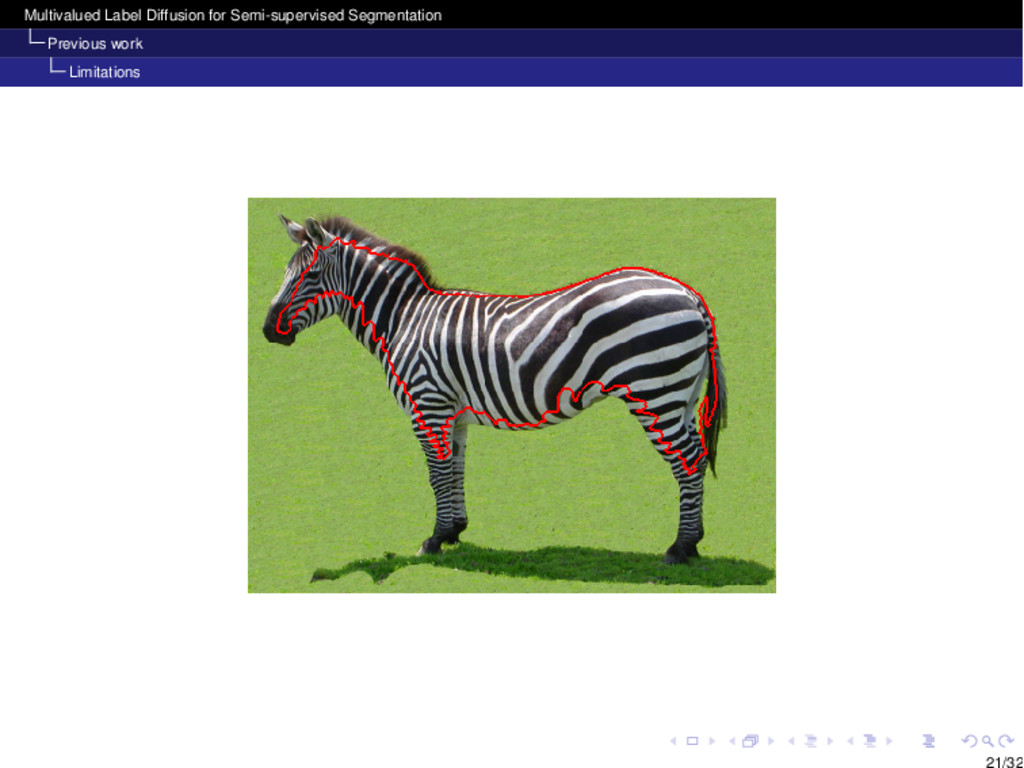
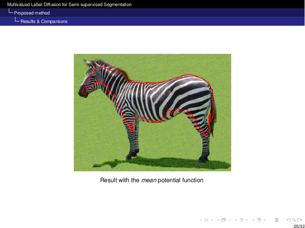
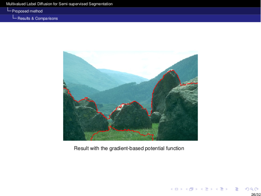
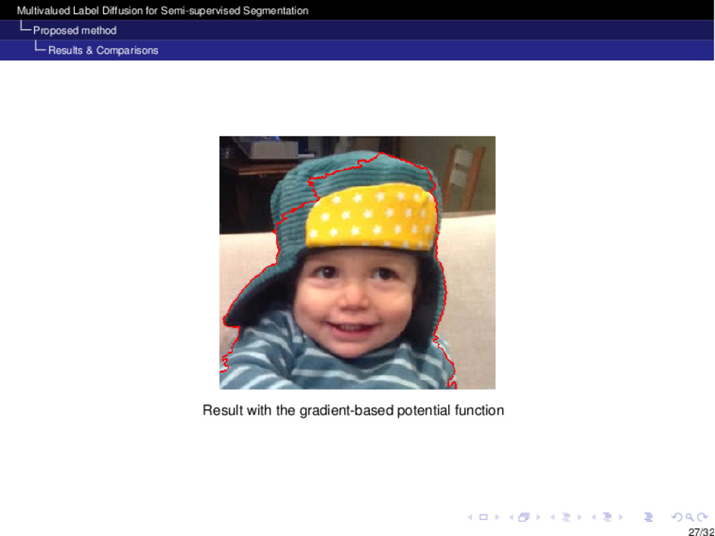
16. Multivalued Label Diffusion for Semi-supervised Segmentation Previous work Region growing diffusion Limitations of the potential function based on the gradient Explanation : The front slows down on a contour, but evolves freely once the contour has been crossed. 16/32
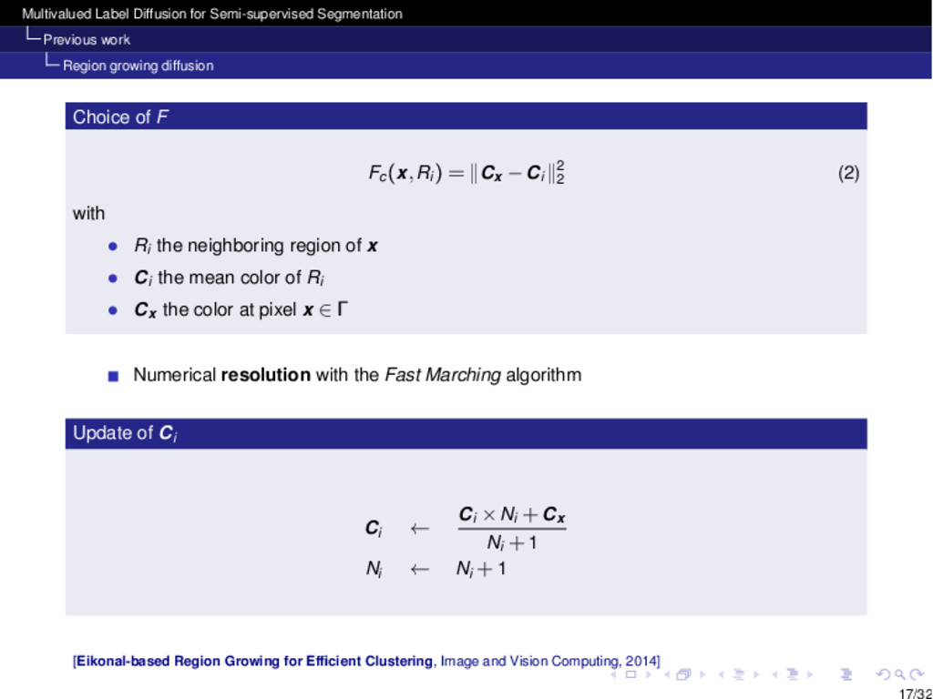
17. Multivalued Label Diffusion for Semi-supervised Segmentation Previous work Region growing diffusion Choice of F Fc ( x , Ri ) = k Cx Ci k2 2 (2) with • Ri the neighboring region of x • Ci the mean color of Ri • Cx the color at pixel x 2 Numerical resolution with the Fast Marching algorithm Update of Ci Ci Ci ⇥ Ni + Cx Ni +1 Ni Ni +1 [Eikonal-based Region Growing for Efficient Clustering, Image and Vision Computing, 2014] 17/32
18. Multivalued Label Diffusion for Semi-supervised Segmentation Previous work Region growing diffusion Advantages : 18/32
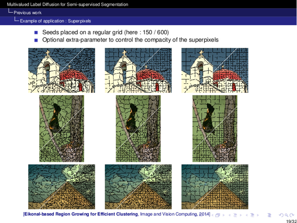
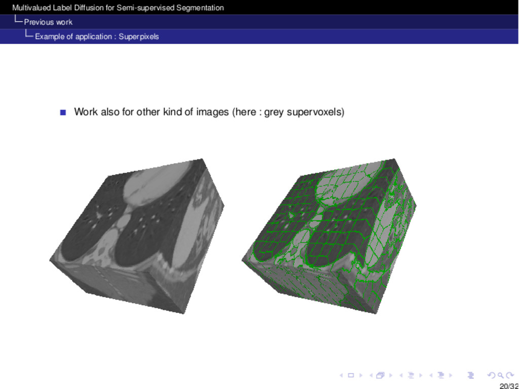
19. Multivalued Label Diffusion for Semi-supervised Segmentation Previous work Example of application : Superpixels Seeds placed on a regular grid (here : 150 / 600) Optional extra-parameter to control the compacity of the superpixels [Eikonal-based Region Growing for Efficient Clustering, Image and Vision Computing, 2014] 19/32
20. Multivalued Label Diffusion for Semi-supervised Segmentation Previous work Example of application : Superpixels Work also for other kind of images (here : grey supervoxels) 20/32
21. Multivalued Label Diffusion for Semi-supervised Segmentation Previous work Limitations 21/32
22. Multivalued Label Diffusion for Semi-supervised Segmentation Previous work Limitations 21/32
23. Multivalued Label Diffusion for Semi-supervised Segmentation Proposed method 1 Previous work Region growing diffusion Example of application : Superpixels Limitations 2 Proposed method Principle Results & Comparisons Texture segmentation 22/32
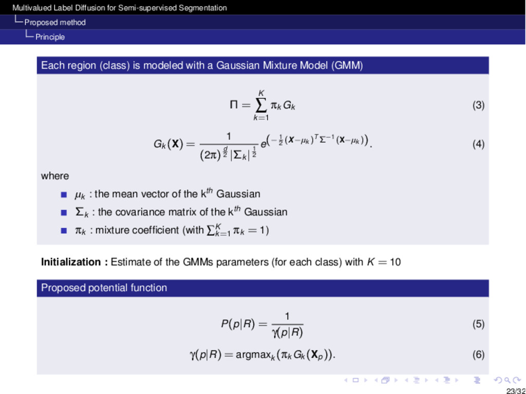
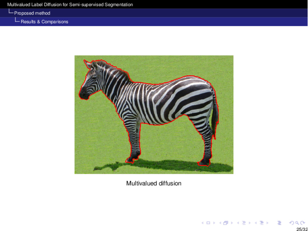
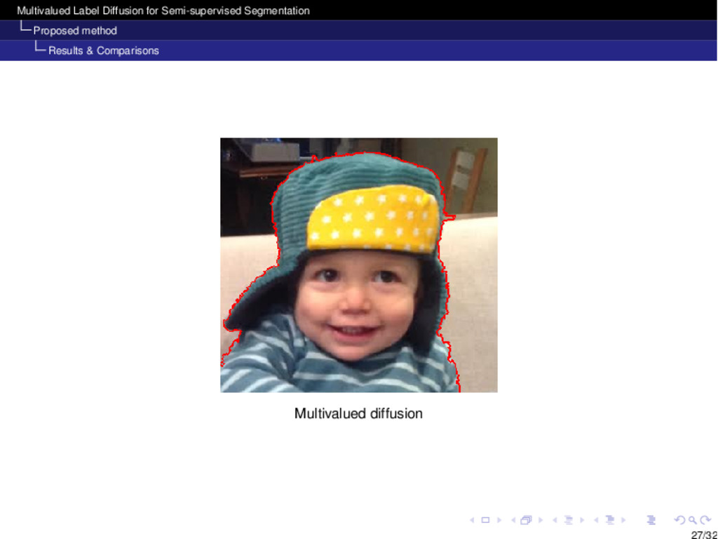
24. Multivalued Label Diffusion for Semi-supervised Segmentation Proposed method Principle Each region (class) is modeled with a Gaussian Mixture Model (GMM) ⇧ = K Â k =1 p k Gk (3) Gk (X) = 1 (2p) d 2 |⌃ k | 1 2 e ( 1 2 ( X µ k )T ⌃ 1 (X µ k )). (4) where µ k : the mean vector of the k th Gaussian ⌃ k : the covariance matrix of the k th Gaussian p k : mixture coefficient (with ÂK k =1 p k = 1) Initialization : Estimate of the GMMs parameters (for each class) with K = 10 Proposed potential function P ( p | R ) = 1 g( p | R ) (5) g( p | R ) = argmax k (p k Gk (X p )). (6) 23/32
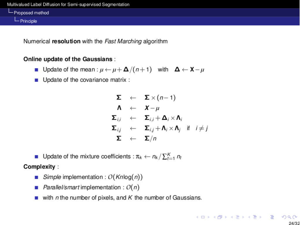
25. Multivalued Label Diffusion for Semi-supervised Segmentation Proposed method Principle Numerical resolution with the Fast Marching algorithm Online update of the Gaussians : Update of the mean : µ µ+ /( n +1) with X µ Update of the covariance matrix : ⌃ ⌃⇥( n 1) ⇤ X µ ⌃ i , i ⌃ i , i + i ⇥⇤ i ⌃ i , j ⌃ i , j +⇤ i ⇥⇤ j if i 6= j ⌃ ⌃/ n Update of the mixture coefficients : p k nk /ÂK t =1 nt Complexity : Simple implementation : O( Kn log( n )) Parallel/smart implementation : O( n ) with n the number of pixels, and K the number of Gaussians. 24/32
26. Multivalued Label Diffusion for Semi-supervised Segmentation Proposed method Results & Comparisons Image with initial seeds 25/32
27. Multivalued Label Diffusion for Semi-supervised Segmentation Proposed method Results & Comparisons PowerWatershed [Couprie et al. , PAMI, 2011] 25/32
28. Multivalued Label Diffusion for Semi-supervised Segmentation Proposed method Results & Comparisons Result with the mean potential function 25/32
29. Multivalued Label Diffusion for Semi-supervised Segmentation Proposed method Results & Comparisons Multivalued diffusion 25/32
30. Multivalued Label Diffusion for Semi-supervised Segmentation Proposed method Results & Comparisons Image with initial seeds 26/32
31. Multivalued Label Diffusion for Semi-supervised Segmentation Proposed method Results & Comparisons PowerWatershed [Couprie et al. , PAMI, 2011] 26/32
32. Multivalued Label Diffusion for Semi-supervised Segmentation Proposed method Results & Comparisons Result with the gradient-based potential function 26/32
33. Multivalued Label Diffusion for Semi-supervised Segmentation Proposed method Results & Comparisons Result with the mean potential function 26/32
34. Multivalued Label Diffusion for Semi-supervised Segmentation Proposed method Results & Comparisons Multivalued diffusion 26/32
35. Multivalued Label Diffusion for Semi-supervised Segmentation Proposed method Results & Comparisons Image with initial seeds 27/32
36. Multivalued Label Diffusion for Semi-supervised Segmentation Proposed method Results & Comparisons PowerWatershed [Couprie et al. , PAMI, 2011] 27/32
37. Multivalued Label Diffusion for Semi-supervised Segmentation Proposed method Results & Comparisons Result with the gradient-based potential function 27/32
38. Multivalued Label Diffusion for Semi-supervised Segmentation Proposed method Results & Comparisons Result with the mean potential function 27/32
39. Multivalued Label Diffusion for Semi-supervised Segmentation Proposed method Results & Comparisons Multivalued diffusion 27/32
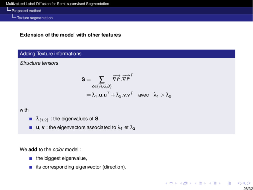
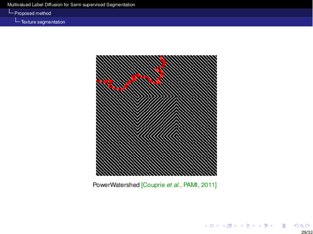
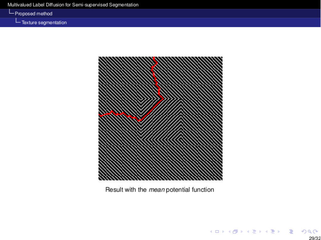
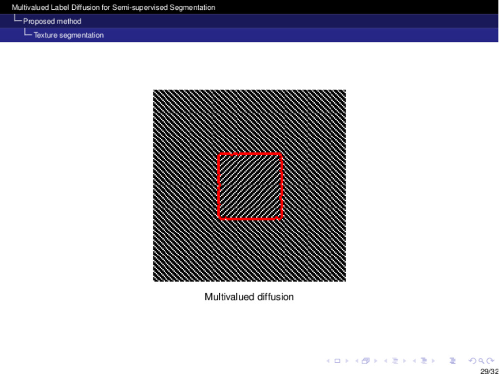
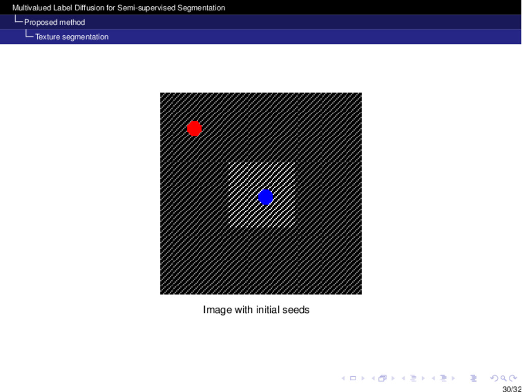
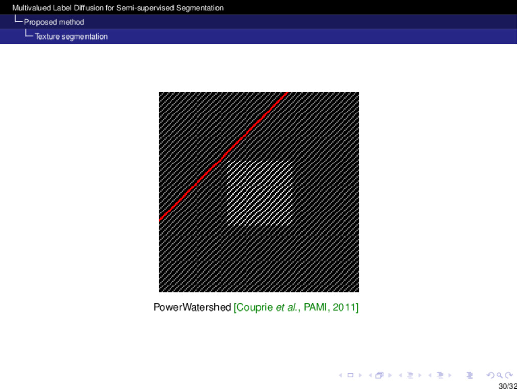
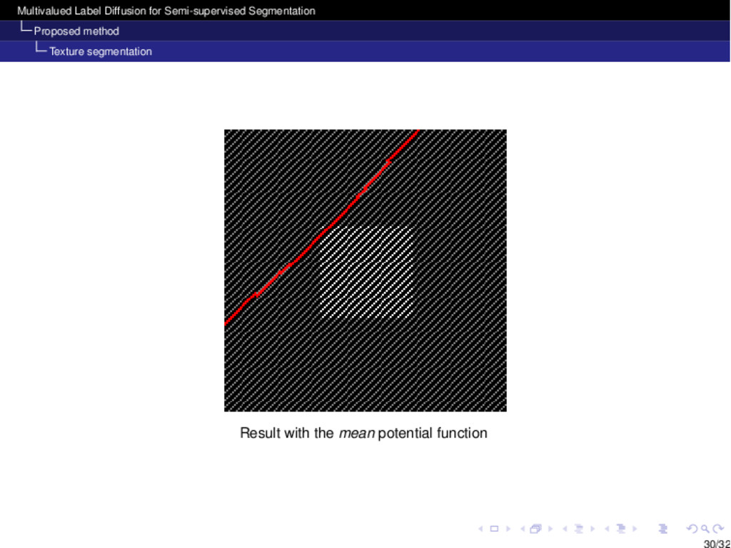
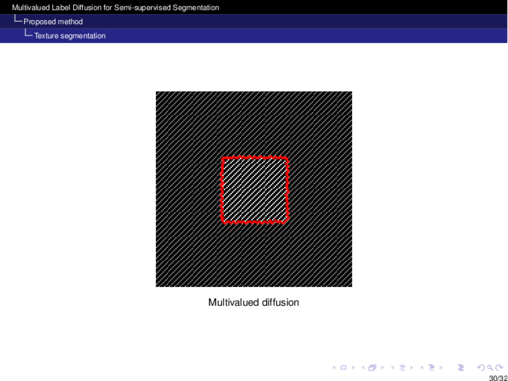
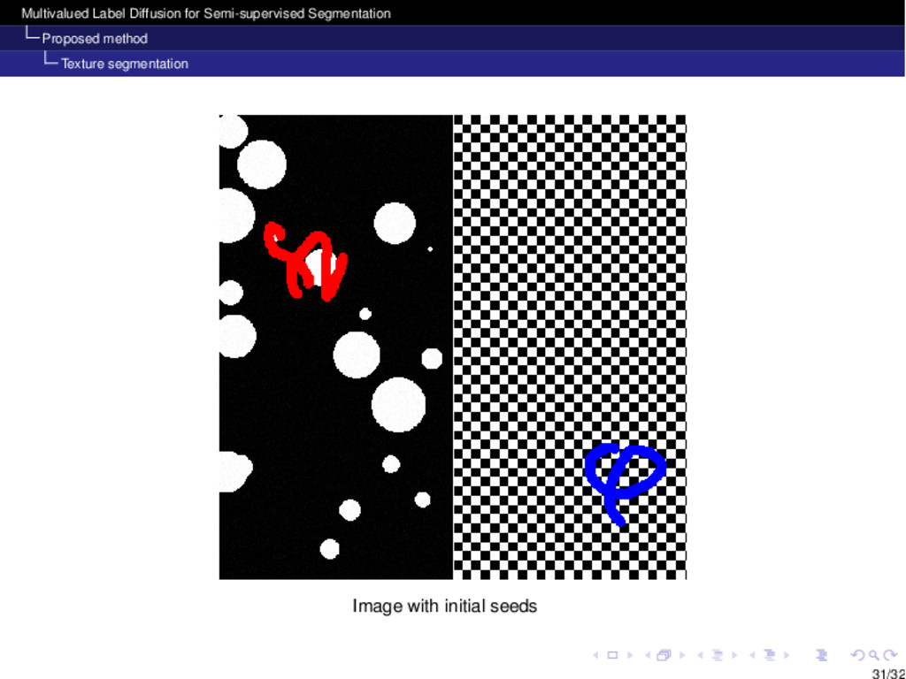
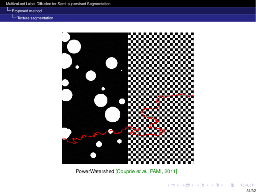
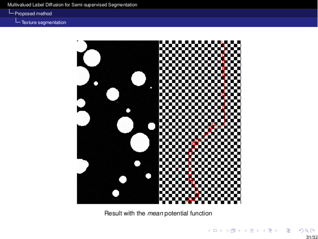
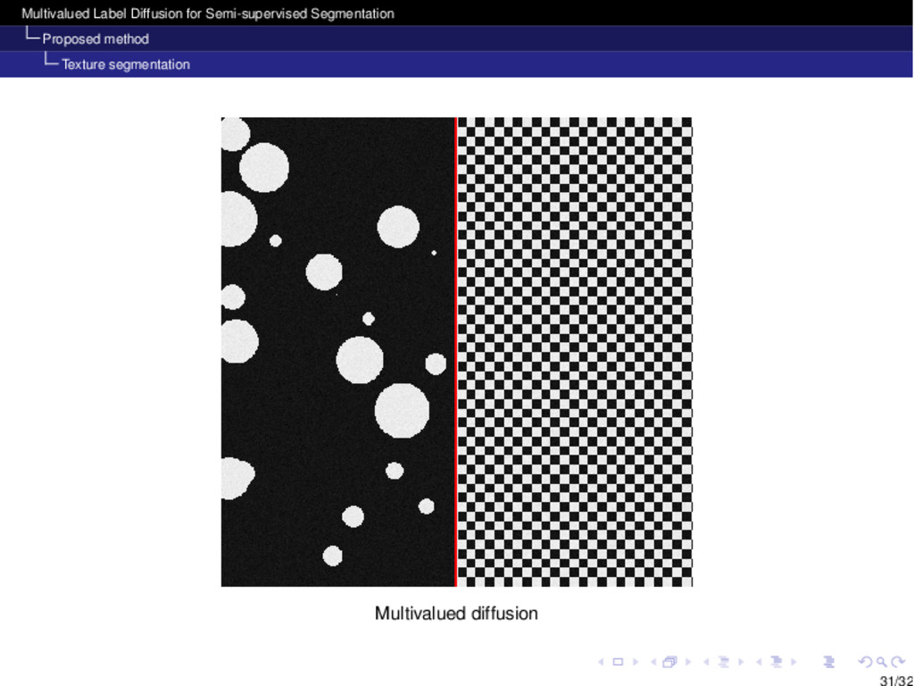
40. Multivalued Label Diffusion for Semi-supervised Segmentation Proposed method Texture segmentation Extension of the model with other features Adding Texture informations Structure tensors S = Â c 2{ R , G , B } ! — Ic. ! — Ic T = l1.u.uT +l2.v.vT avec l1 > l2 with l {1,2} : the eigenvalues of S u, v : the eigenvectors associated to l1 et l2 We add to the color model : the biggest eigenvalue, its corresponding eigenvector (direction). 28/32
41. Multivalued Label Diffusion for Semi-supervised Segmentation Proposed method Texture segmentation Image with initial seeds 29/32
42. Multivalued Label Diffusion for Semi-supervised Segmentation Proposed method Texture segmentation PowerWatershed [Couprie et al. , PAMI, 2011] 29/32
43. Multivalued Label Diffusion for Semi-supervised Segmentation Proposed method Texture segmentation Result with the mean potential function 29/32
44. Multivalued Label Diffusion for Semi-supervised Segmentation Proposed method Texture segmentation Multivalued diffusion 29/32
45. Multivalued Label Diffusion for Semi-supervised Segmentation Proposed method Texture segmentation Image with initial seeds 30/32
46. Multivalued Label Diffusion for Semi-supervised Segmentation Proposed method Texture segmentation PowerWatershed [Couprie et al. , PAMI, 2011] 30/32
47. Multivalued Label Diffusion for Semi-supervised Segmentation Proposed method Texture segmentation Result with the mean potential function 30/32
48. Multivalued Label Diffusion for Semi-supervised Segmentation Proposed method Texture segmentation Multivalued diffusion 30/32
49. Multivalued Label Diffusion for Semi-supervised Segmentation Proposed method Texture segmentation Image with initial seeds 31/32
50. Multivalued Label Diffusion for Semi-supervised Segmentation Proposed method Texture segmentation PowerWatershed [Couprie et al. , PAMI, 2011] 31/32
51. Multivalued Label Diffusion for Semi-supervised Segmentation Proposed method Texture segmentation Result with the mean potential function 31/32
52. Multivalued Label Diffusion for Semi-supervised Segmentation Proposed method Texture segmentation Multivalued diffusion 31/32
53. Multivalued Label Diffusion for Semi-supervised Segmentation Proposed method Texture segmentation Thanks for your attention Papers and codes available at : https ://sites.google.com/site/pierrebuyssens 32/32