4. Graph signal p-Laplacian regularization 5. Mathematical Morphology 6. From continuous MM to Active contours on graphs Olivier L´ ezoray Graph signal processing : from images to arbitrary graphs 2 / 96
4. Graph signal p-Laplacian regularization 5. Mathematical Morphology 6. From continuous MM to Active contours on graphs Olivier L´ ezoray Graph signal processing : from images to arbitrary graphs 3 / 96
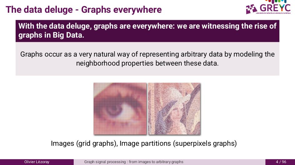
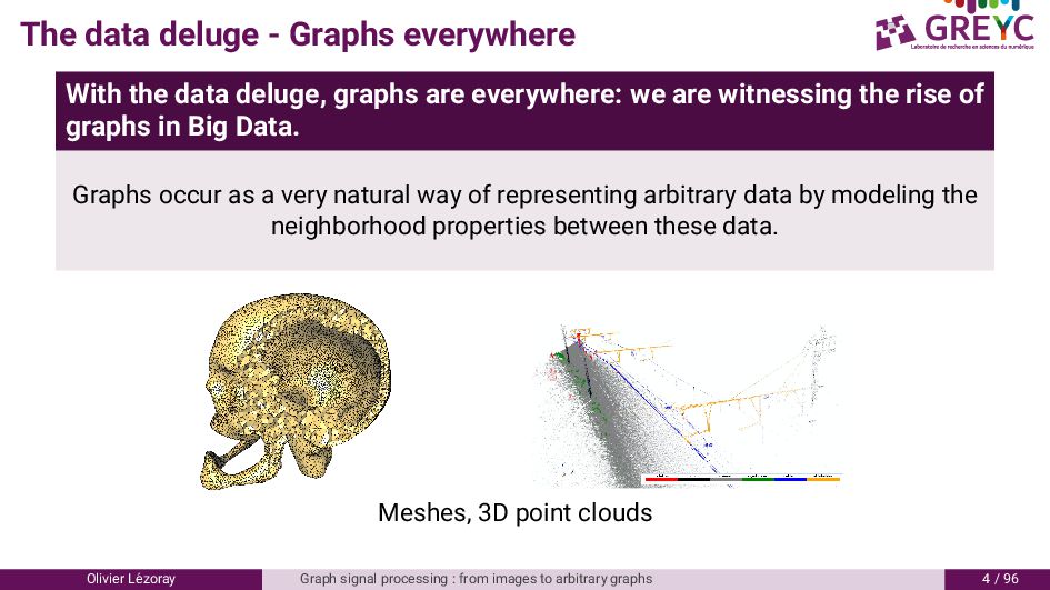
graphs are everywhere: we are witnessing the rise of graphs in Big Data. Graphs occur as a very natural way of representing arbitrary data by modeling the neighborhood properties between these data. Olivier L´ ezoray Graph signal processing : from images to arbitrary graphs 4 / 96
graphs are everywhere: we are witnessing the rise of graphs in Big Data. Graphs occur as a very natural way of representing arbitrary data by modeling the neighborhood properties between these data. Images (grid graphs), Image partitions (superpixels graphs) Olivier L´ ezoray Graph signal processing : from images to arbitrary graphs 4 / 96
graphs are everywhere: we are witnessing the rise of graphs in Big Data. Graphs occur as a very natural way of representing arbitrary data by modeling the neighborhood properties between these data. Meshes, 3D point clouds Olivier L´ ezoray Graph signal processing : from images to arbitrary graphs 4 / 96
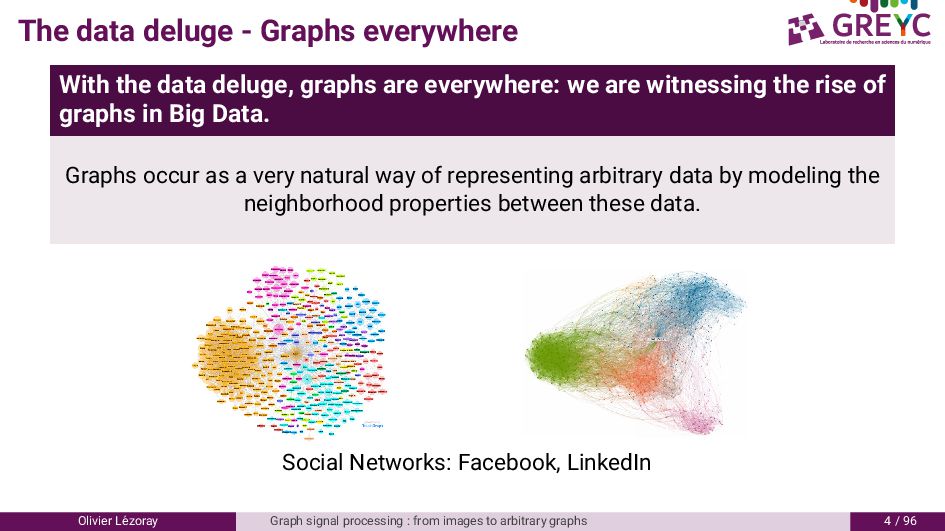
graphs are everywhere: we are witnessing the rise of graphs in Big Data. Graphs occur as a very natural way of representing arbitrary data by modeling the neighborhood properties between these data. Social Networks: Facebook, LinkedIn Olivier L´ ezoray Graph signal processing : from images to arbitrary graphs 4 / 96
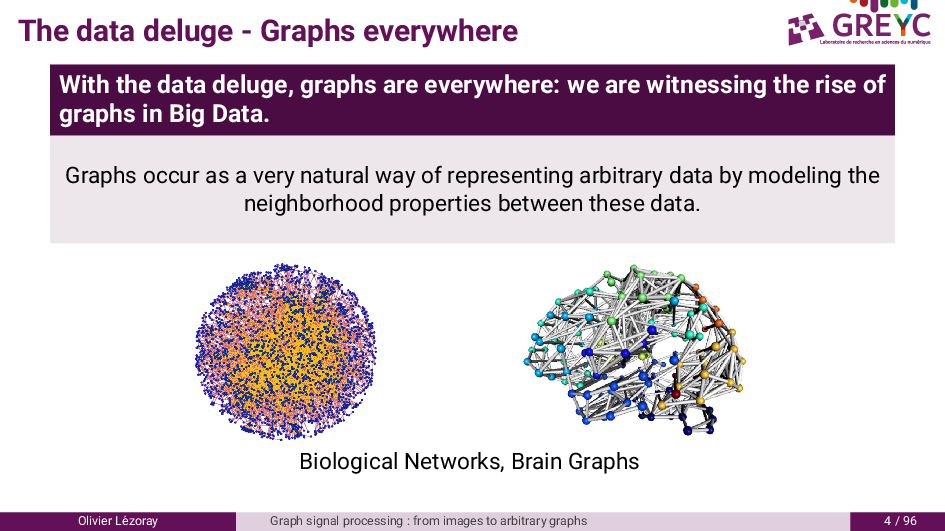
graphs are everywhere: we are witnessing the rise of graphs in Big Data. Graphs occur as a very natural way of representing arbitrary data by modeling the neighborhood properties between these data. Biological Networks, Brain Graphs Olivier L´ ezoray Graph signal processing : from images to arbitrary graphs 4 / 96
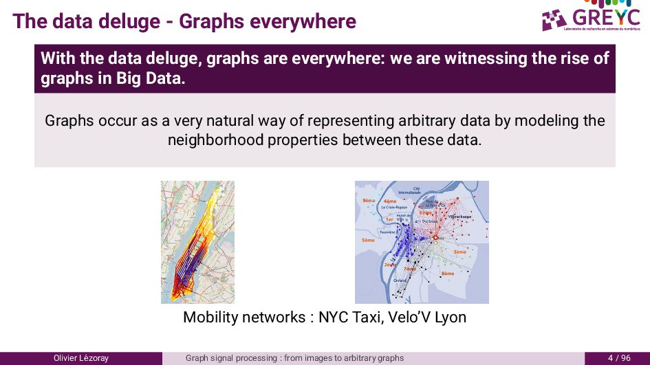
graphs are everywhere: we are witnessing the rise of graphs in Big Data. Graphs occur as a very natural way of representing arbitrary data by modeling the neighborhood properties between these data. Mobility networks : NYC Taxi, Velo’V Lyon Olivier L´ ezoray Graph signal processing : from images to arbitrary graphs 4 / 96
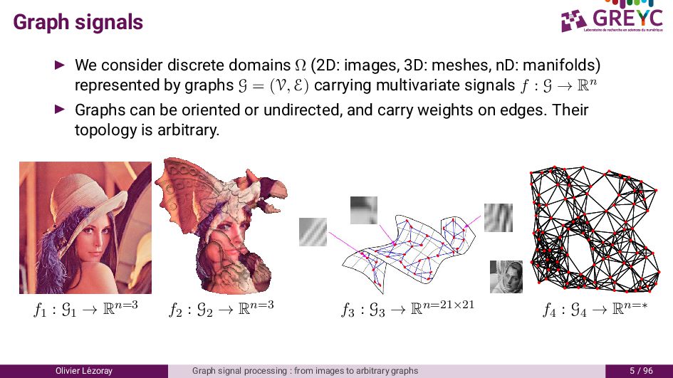
3D: meshes, nD: manifolds) represented by graphs G = (V, E) carrying multivariate signals f : G → Rn ▶ Graphs can be oriented or undirected, and carry weights on edges. Their topology is arbitrary. f1 : G1 → Rn=3 f2 : G2 → Rn=3 f3 : G3 → Rn=21×21 f4 : G4 → Rn=∗ Olivier L´ ezoray Graph signal processing : from images to arbitrary graphs 5 / 96
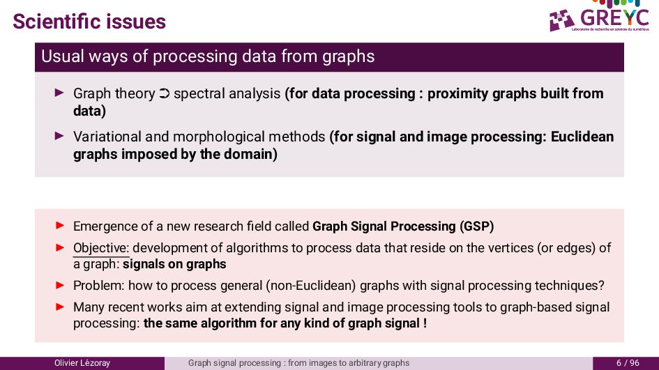
Graph theory ➲ spectral analysis (for data processing : proximity graphs built from data) ▶ Variational and morphological methods (for signal and image processing: Euclidean graphs imposed by the domain) ▶ Emergence of a new research field called Graph Signal Processing (GSP) ▶ Objective: development of algorithms to process data that reside on the vertices (or edges) of a graph: signals on graphs ▶ Problem: how to process general (non-Euclidean) graphs with signal processing techniques? ▶ Many recent works aim at extending signal and image processing tools to graph-based signal processing: the same algorithm for any kind of graph signal ! Olivier L´ ezoray Graph signal processing : from images to arbitrary graphs 6 / 96
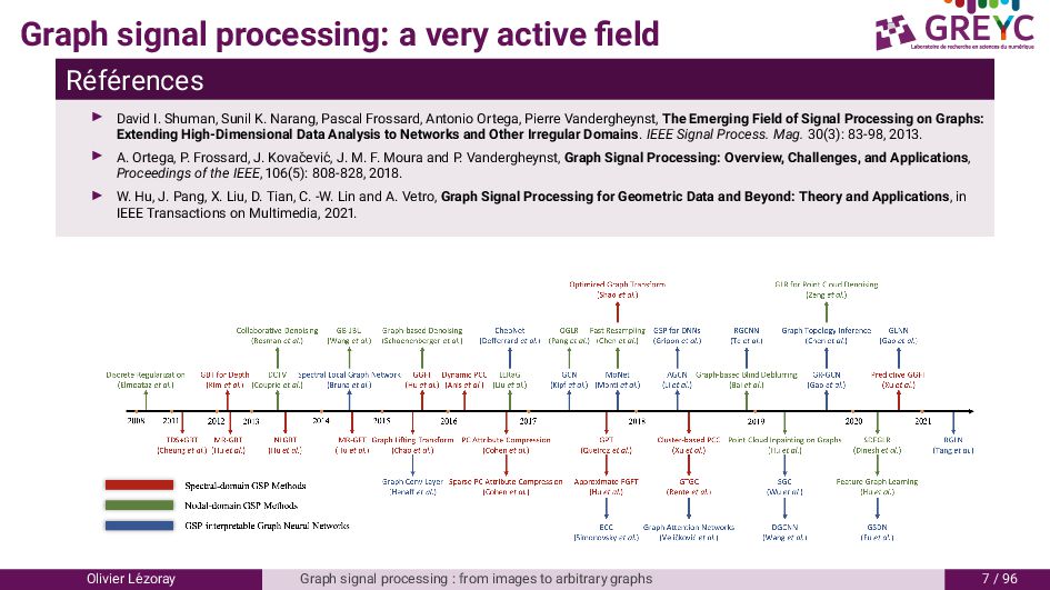
▶ David I. Shuman, Sunil K. Narang, Pascal Frossard, Antonio Ortega, Pierre Vandergheynst, The Emerging Field of Signal Processing on Graphs: Extending High-Dimensional Data Analysis to Networks and Other Irregular Domains. IEEE Signal Process. Mag. 30(3): 83-98, 2013. ▶ A. Ortega, P. Frossard, J. Kovaˇ cevi´ c, J. M. F. Moura and P. Vandergheynst, Graph Signal Processing: Overview, Challenges, and Applications, Proceedings of the IEEE, 106(5): 808-828, 2018. ▶ W. Hu, J. Pang, X. Liu, D. Tian, C. -W. Lin and A. Vetro, Graph Signal Processing for Geometric Data and Beyond: Theory and Applications, in IEEE Transactions on Multimedia, 2021. Olivier L´ ezoray Graph signal processing : from images to arbitrary graphs 7 / 96
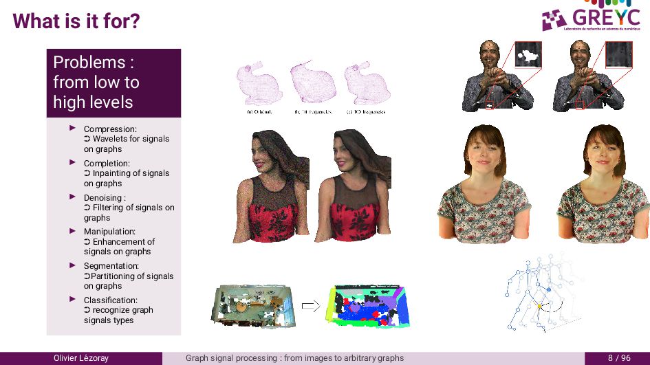
levels ▶ Compression: ➲ Wavelets for signals on graphs ▶ Completion: ➲ Inpainting of signals on graphs ▶ Denoising : ➲ Filtering of signals on graphs ▶ Manipulation: ➲ Enhancement of signals on graphs ▶ Segmentation: ➲Partitioning of signals on graphs ▶ Classification: ➲ recognize graph signals types Olivier L´ ezoray Graph signal processing : from images to arbitrary graphs 8 / 96
4. Graph signal p-Laplacian regularization 5. Mathematical Morphology 6. From continuous MM to Active contours on graphs Olivier L´ ezoray Graph signal processing : from images to arbitrary graphs 9 / 96
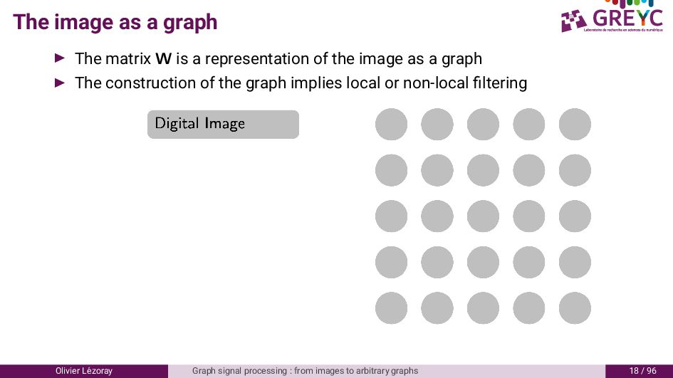
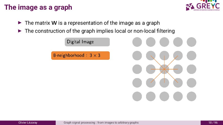
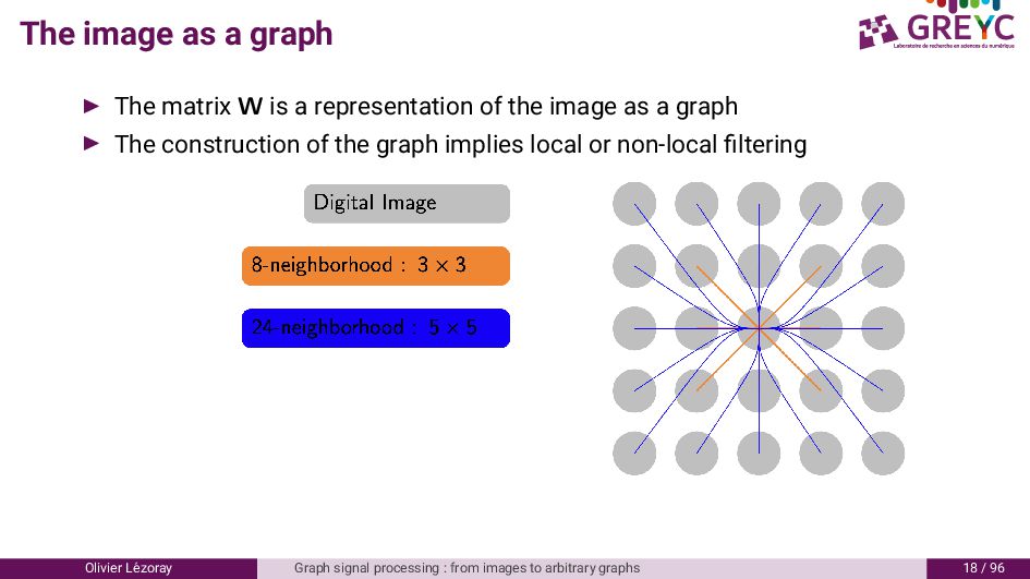
a representation of the image as a graph ▶ The construction of the graph implies local or non-local filtering Olivier L´ ezoray Graph signal processing : from images to arbitrary graphs 18 / 96
a representation of the image as a graph ▶ The construction of the graph implies local or non-local filtering Olivier L´ ezoray Graph signal processing : from images to arbitrary graphs 18 / 96
a representation of the image as a graph ▶ The construction of the graph implies local or non-local filtering Olivier L´ ezoray Graph signal processing : from images to arbitrary graphs 18 / 96
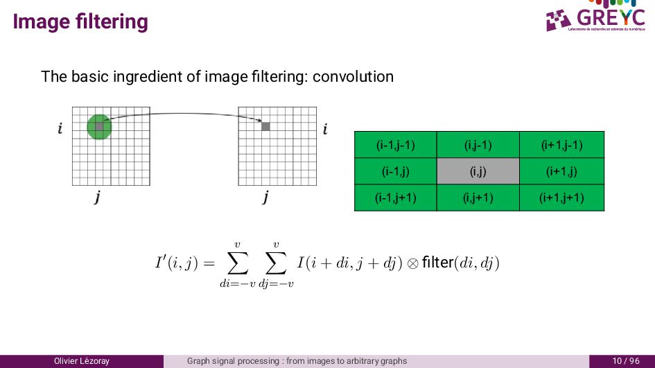
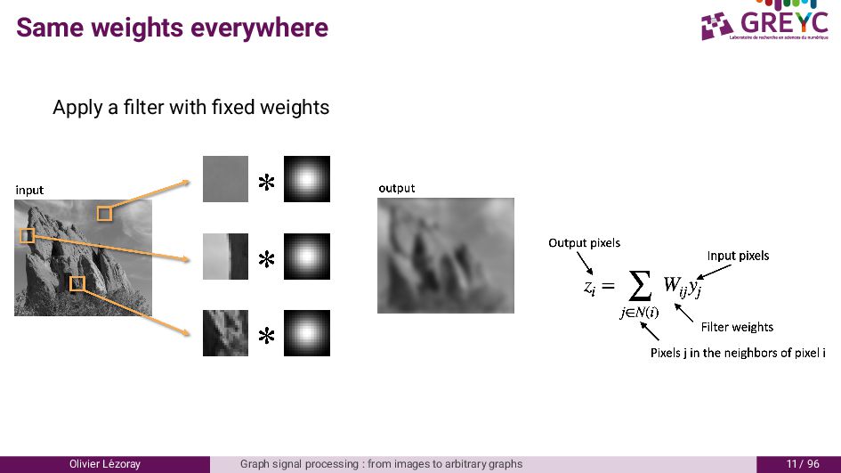
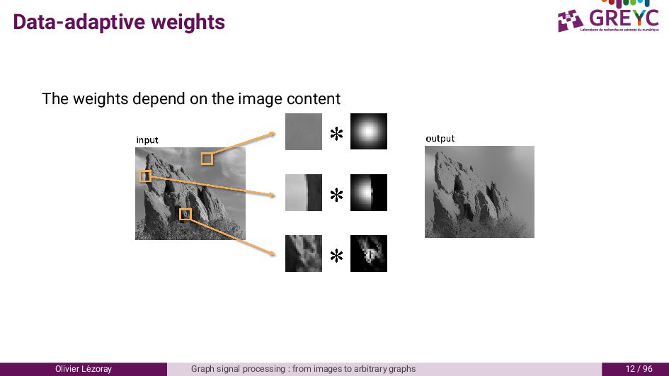
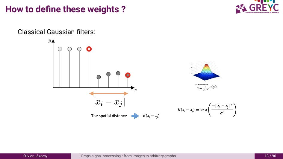
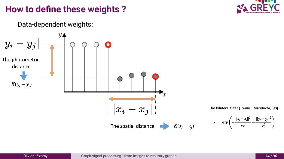
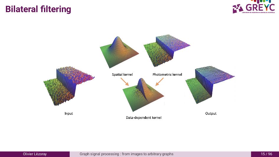
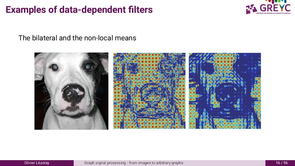
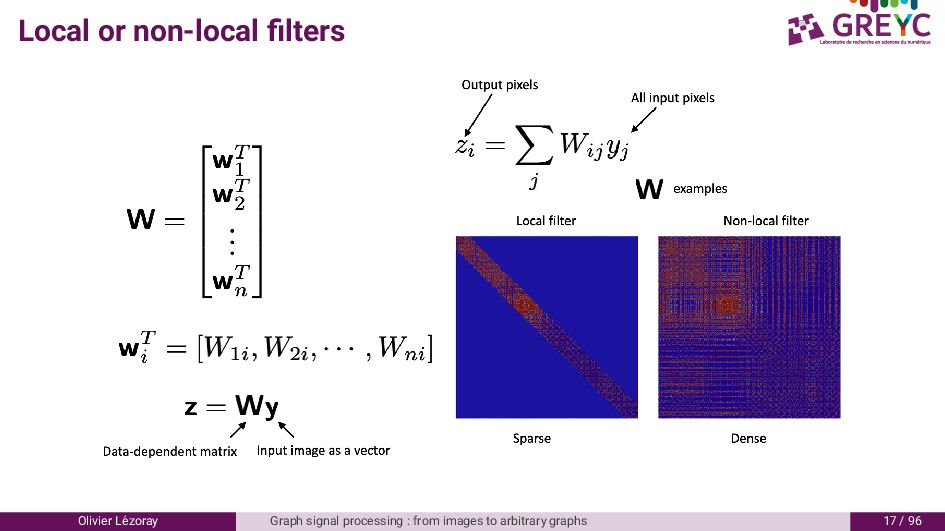
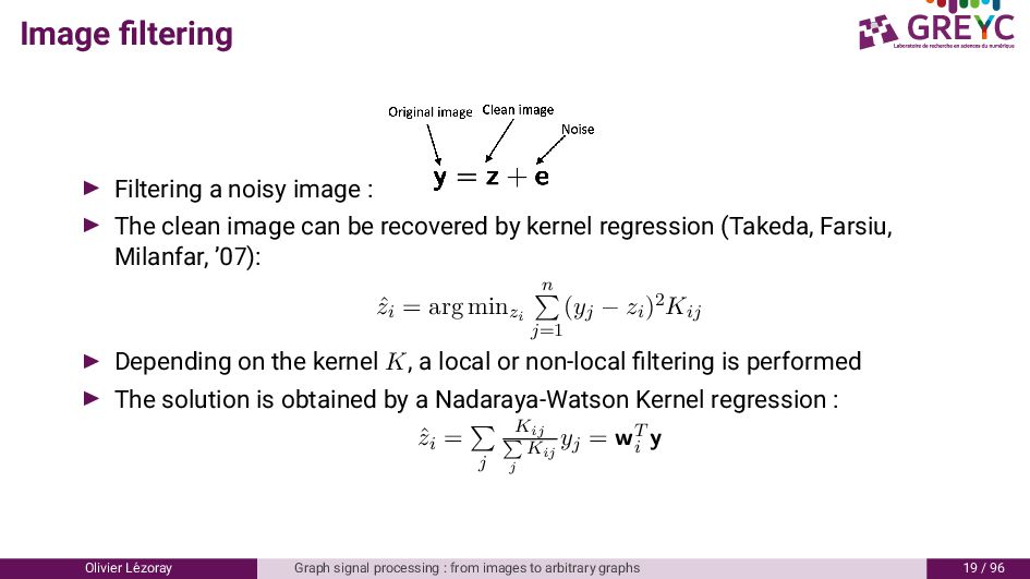
clean image can be recovered by kernel regression (Takeda, Farsiu, Milanfar, ’07): ˆ zi = arg minzi n j=1 (yj − zi)2Kij ▶ Depending on the kernel K, a local or non-local filtering is performed ▶ The solution is obtained by a Nadaraya-Watson Kernel regression : ˆ zi = j Kij j Kij yj = wT i y Olivier L´ ezoray Graph signal processing : from images to arbitrary graphs 19 / 96
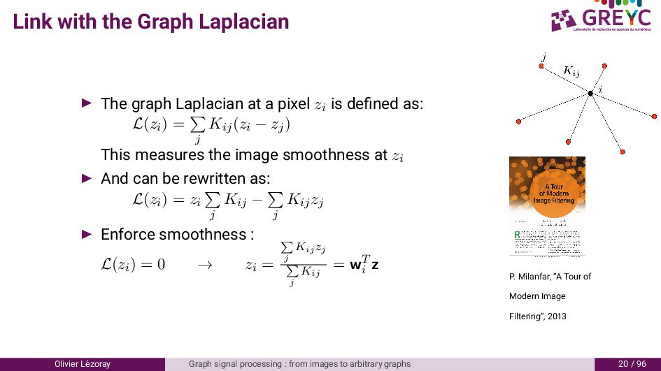
a pixel zi is defined as: L(zi) = j Kij(zi − zj) This measures the image smoothness at zi ▶ And can be rewritten as: L(zi) = zi j Kij − j Kijzj ▶ Enforce smoothness : L(zi) = 0 → zi = j Kij zj j Kij = wT i z P. Milanfar, ”A Tour of Modern Image Filtering”, 2013 Olivier L´ ezoray Graph signal processing : from images to arbitrary graphs 20 / 96
as a data-dependent kernel regression on a graph ▶ The topology of the graph implies local or non-local processing ▶ The weights of the graph imply a data-dependent processing ▶ However, images are very specific data organized in a grid on a Euclidean domain ▶ Can we generalize this to signals defined on non-Euclidean domains ? ▶ Can we also generalize other image processing tasks (segmentation, interpolation) to signals on arbitrary graphs ? Olivier L´ ezoray Graph signal processing : from images to arbitrary graphs 21 / 96
4. Graph signal p-Laplacian regularization 5. Mathematical Morphology 6. From continuous MM to Active contours on graphs Olivier L´ ezoray Graph signal processing : from images to arbitrary graphs 22 / 96
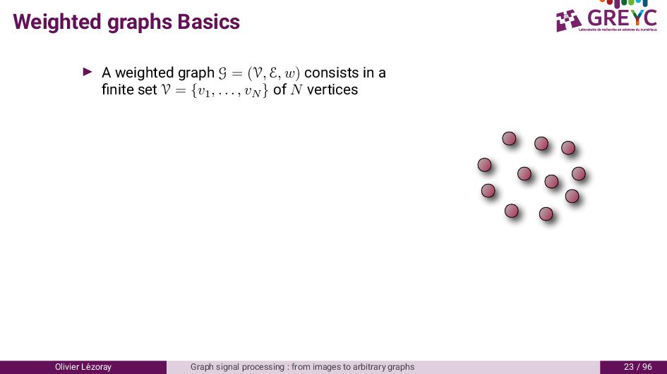
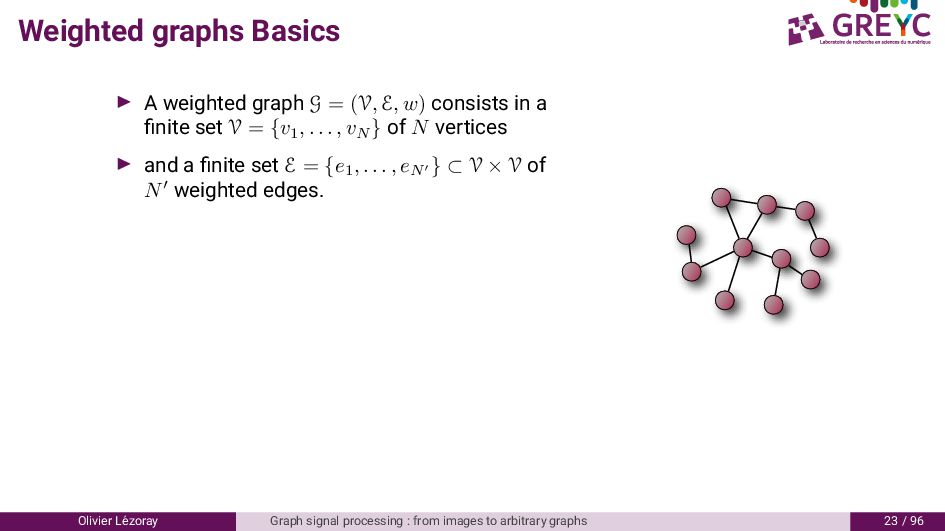
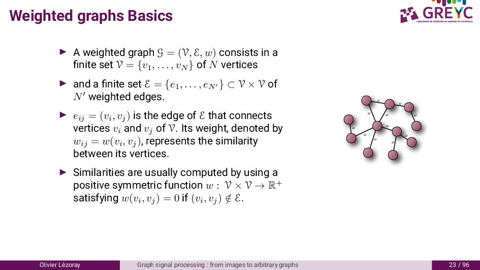
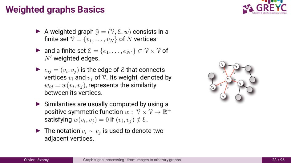
E, w) consists in a finite set V = {v1 , . . . , vN } of N vertices ▶ and a finite set E = {e1 , . . . , eN′ } ⊂ V × V of N′ weighted edges. Olivier L´ ezoray Graph signal processing : from images to arbitrary graphs 23 / 96
E, w) consists in a finite set V = {v1 , . . . , vN } of N vertices ▶ and a finite set E = {e1 , . . . , eN′ } ⊂ V × V of N′ weighted edges. ▶ eij = (vi , vj ) is the edge of E that connects vertices vi and vj of V. Its weight, denoted by wij = w(vi , vj ), represents the similarity between its vertices. ▶ Similarities are usually computed by using a positive symmetric function w : V × V → R+ satisfying w(vi , vj ) = 0 if (vi , vj ) / ∈ E. w w w w w w w w w w w Olivier L´ ezoray Graph signal processing : from images to arbitrary graphs 23 / 96
E, w) consists in a finite set V = {v1 , . . . , vN } of N vertices ▶ and a finite set E = {e1 , . . . , eN′ } ⊂ V × V of N′ weighted edges. ▶ eij = (vi , vj ) is the edge of E that connects vertices vi and vj of V. Its weight, denoted by wij = w(vi , vj ), represents the similarity between its vertices. ▶ Similarities are usually computed by using a positive symmetric function w : V × V → R+ satisfying w(vi , vj ) = 0 if (vi , vj ) / ∈ E. ▶ The notation vi ∼ vj is used to denote two adjacent vertices. Olivier L´ ezoray Graph signal processing : from images to arbitrary graphs 23 / 96
the Hilbert spaces of graph signals: real-valued functions defined on the vertices or the edges of a graph G. ▶ A function f : V → R of H(V) assigns a real value xi = f(vi) to vi ∈ V. ▶ By analogy with functional analysis on continuous spaces, the integral of a function f ∈ H(V), over the set of vertices V, is defined as V f = V f ▶ Both spaces H(V) and H(E) are endowed with the usual inner products: ⟨f, h⟩H(V) = vi∈V f(vi)h(vi), where f, h : V → R ⟨F, H⟩H(E) = vi∈V vj∼vi F(vi, vj)H(vi, vj) where F, H : E → R Olivier L´ ezoray Graph signal processing : from images to arbitrary graphs 24 / 96
of classical continuous differential geometry. The difference operator of f, dw : H(V) → H(E), is defined on an edge eij = (vi, vj) ∈ E by: (dwf)(eij) = (dwf)(vi, vj) = w(vi, vj)1/2(f(vj) − f(vi)) . (1) The adjoint of the difference operator, d∗ w : H(E) → H(V), is a linear operator defined by ⟨dwf, H⟩H(E) = ⟨f, d∗ w H⟩H(V) and expressed by (d∗ w H)(vi) = −divw(H)(vi) = vj∼vi w(vi, vj)1/2(H(vj, vi) − H(vi, vj)) . (2) Olivier L´ ezoray Graph signal processing : from images to arbitrary graphs 25 / 96
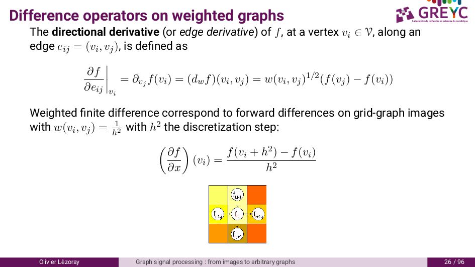
derivative) of f, at a vertex vi ∈ V, along an edge eij = (vi, vj), is defined as ∂f ∂eij vi = ∂vj f(vi) = (dwf)(vi, vj) = w(vi, vj)1/2(f(vj) − f(vi)) Weighted finite difference correspond to forward differences on grid-graph images with w(vi, vj) = 1 h2 with h2 the discretization step: ∂f ∂x (vi) = f(vi + h2) − f(vi) h2 Olivier L´ ezoray Graph signal processing : from images to arbitrary graphs 26 / 96
f ∈ H(V), at a vertex vi ∈ V, is the vector operator defined by (∇wf)(vi ) = [(dwf)(vi, vj) : vj ∈ V]T . (3) ➲ The gradient considers all vertices vj ∈ V and not only vj ∼ vi. The Lp norm of this vector represents the local variation of the function f at a vertex of the graph (It is a semi-norm for p ≥ 1): ∥(∇wf)(vi )∥p = vj∼vi wp/2 ij f(vj)−f(vi) p 1/p . (4) Olivier L´ ezoray Graph signal processing : from images to arbitrary graphs 27 / 96
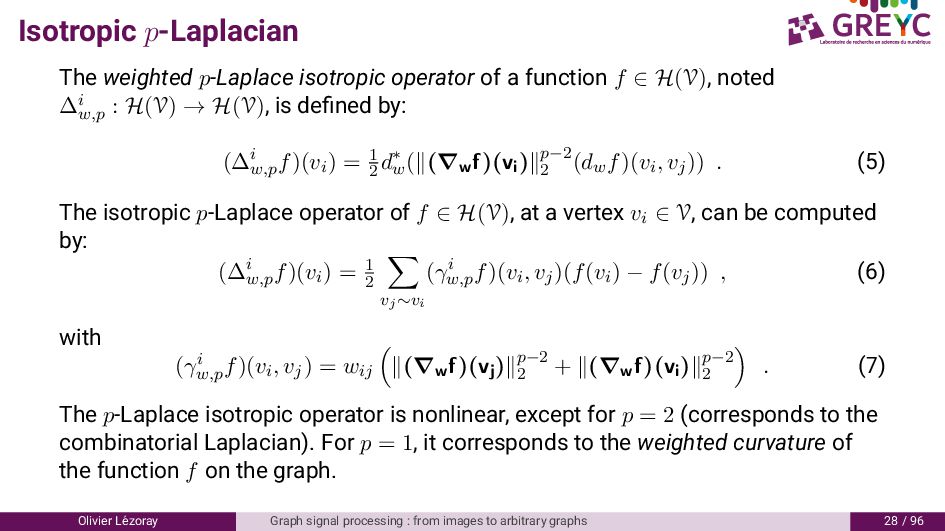
f ∈ H(V), noted ∆i w,p : H(V) → H(V), is defined by: (∆i w,p f)(vi) = 1 2 d∗ w (∥(∇wf)(vi )∥p−2 2 (dwf)(vi, vj)) . (5) The isotropic p-Laplace operator of f ∈ H(V), at a vertex vi ∈ V, can be computed by: (∆i w,p f)(vi) = 1 2 vj∼vi (γi w,p f)(vi, vj)(f(vi) − f(vj)) , (6) with (γi w,p f)(vi, vj) = wij ∥(∇wf)(vj )∥p−2 2 + ∥(∇wf)(vi )∥p−2 2 . (7) The p-Laplace isotropic operator is nonlinear, except for p = 2 (corresponds to the combinatorial Laplacian). For p = 1, it corresponds to the weighted curvature of the function f on the graph. Olivier L´ ezoray Graph signal processing : from images to arbitrary graphs 28 / 96
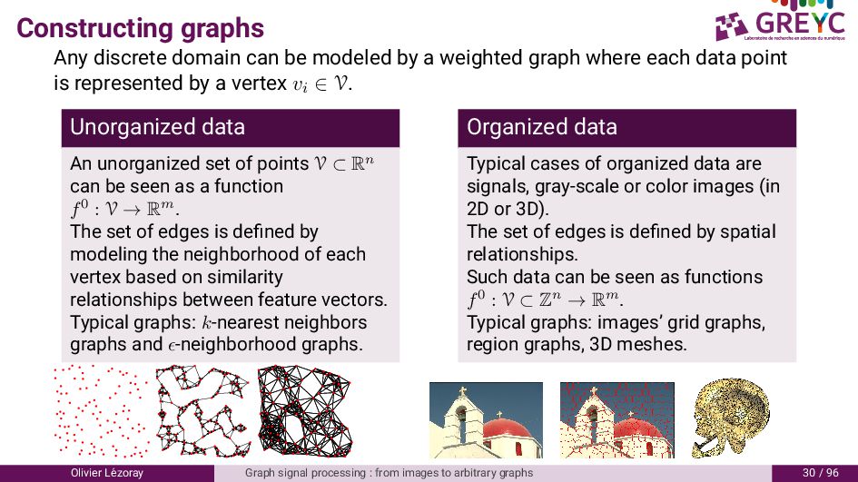
weighted graph where each data point is represented by a vertex vi ∈ V. Unorganized data An unorganized set of points V ⊂ Rn can be seen as a function f0 : V → Rm. The set of edges is defined by modeling the neighborhood of each vertex based on similarity relationships between feature vectors. Typical graphs: k-nearest neighbors graphs and ϵ-neighborhood graphs. Organized data Typical cases of organized data are signals, gray-scale or color images (in 2D or 3D). The set of edges is defined by spatial relationships. Such data can be seen as functions f0 : V ⊂ Zn → Rm. Typical graphs: images’ grid graphs, region graphs, 3D meshes. Olivier L´ ezoray Graph signal processing : from images to arbitrary graphs 30 / 96
Rm, similarity relationship between data can be incorporated within edges weights according to a measure of similarity g : E → [0, 1] with w(eij) = g(eij), ∀eij ∈ E. Each vertex vi is associated with a feature vector Ff0 τ : V → Rm×q where q corresponds to this vector size: Ff0 τ (vi) = f0(vj) : vj ∈ Nτ (vi) ∪ {vi } T (11) with Nτ (vi) = vj ∈ V \ {vi } : µ(vi, vj) ≤ τ . For an edge eij and a distance measure ρ : Rm×q×Rm×q → R associated to Ff0 τ , we can have: g1(eij) =1 (unweighted case) , g2(eij) = exp −ρ Ff0 τ (vi), Ff0 τ (vj) 2/σ2 with σ > 0 , g3(eij) =1/ 1 + ρ Ff0 τ (vi), Ff0 τ (vj) (12) Olivier L´ ezoray Graph signal processing : from images to arbitrary graphs 31 / 96
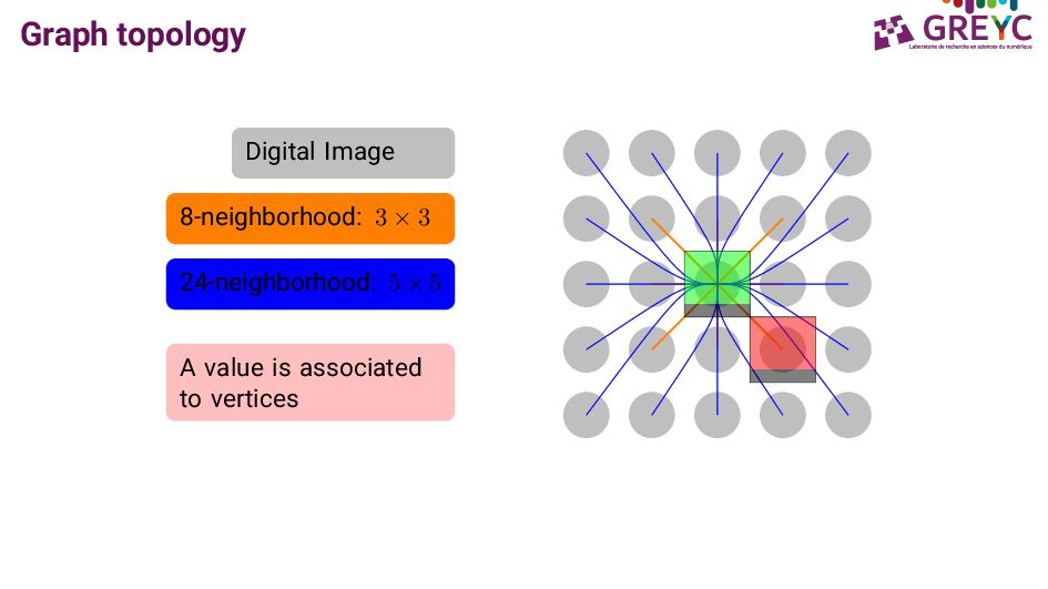
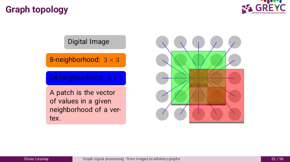
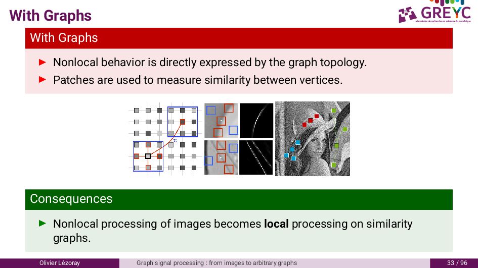
× 5 A value is associated to vertices A patch is the vector of values in a given neighborhood of a ver- tex. Olivier L´ ezoray Graph signal processing : from images to arbitrary graphs 32 / 96
by the graph topology. ▶ Patches are used to measure similarity between vertices. Consequences ▶ Nonlocal processing of images becomes local processing on similarity graphs. Olivier L´ ezoray Graph signal processing : from images to arbitrary graphs 33 / 96
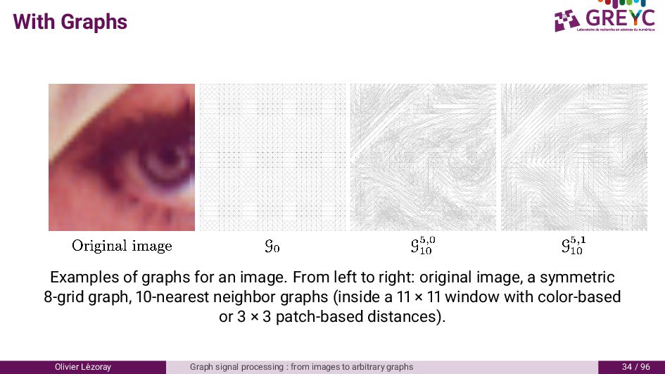
to right: original image, a symmetric 8-grid graph, 10-nearest neighbor graphs (inside a 11 × 11 window with color-based or 3 × 3 patch-based distances). Olivier L´ ezoray Graph signal processing : from images to arbitrary graphs 34 / 96
4. Graph signal p-Laplacian regularization 5. Mathematical Morphology 6. From continuous MM to Active contours on graphs Olivier L´ ezoray Graph signal processing : from images to arbitrary graphs 35 / 96
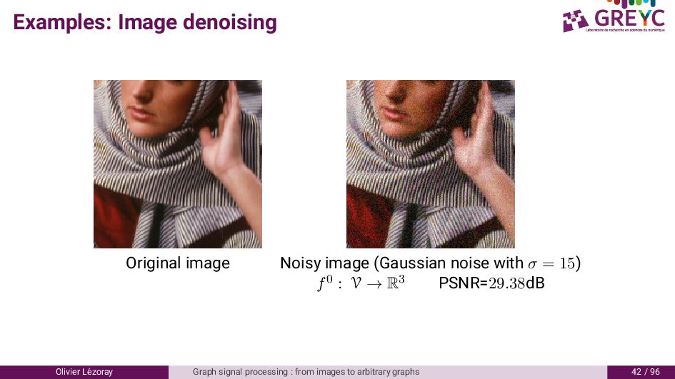
R be the noisy version of a clean graph signal g : V → R defined on the vertices of a weighted graph G = (V, E, w). To recover g, seek for a function f : V → R regular enough on G, and close enough to f0, with the following variational problem: g ≈ min f:V→R E∗ w,p (f, f0, λ) = R∗ w,p (f) + λ 2 ∥f − f0∥2 2 , (13) where the regularization functional R∗ w,p : H(V) → R can correspond to an isotropic Ri w,p or an anisotropic Ra w,p functionnal. Olivier L´ ezoray Graph signal processing : from images to arbitrary graphs 36 / 96
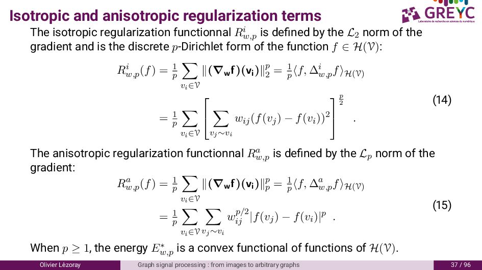
w,p is defined by the L2 norm of the gradient and is the discrete p-Dirichlet form of the function f ∈ H(V): Ri w,p (f) = 1 p vi∈V ∥(∇wf)(vi )∥p 2 = 1 p ⟨f, ∆i w,p f⟩H(V) = 1 p vi∈V vj∼vi wij(f(vj) − f(vi))2 p 2 . (14) The anisotropic regularization functionnal Ra w,p is defined by the Lp norm of the gradient: Ra w,p (f) = 1 p vi∈V ∥(∇wf)(vi )∥p p = 1 p ⟨f, ∆a w,p f⟩H(V) = 1 p vi∈V vj∼vi wp/2 ij |f(vj) − f(vi)|p . (15) When p ≥ 1, the energy E∗ w,p is a convex functional of functions of H(V). Olivier L´ ezoray Graph signal processing : from images to arbitrary graphs 37 / 96
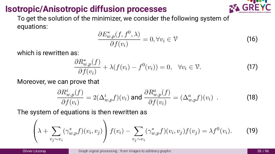
we consider the following system of equations: ∂E∗ w,p (f, f0, λ) ∂f(vi) = 0, ∀vi ∈ V (16) which is rewritten as: ∂R∗ w,p (f) ∂f(vi) + λ(f(vi) − f0(vi)) = 0, ∀vi ∈ V. (17) Moreover, we can prove that ∂Ri w,p (f) ∂f(vi) = 2(∆i w,p f)(vi) and ∂Ra w,p (f) ∂f(vi) = (∆a w,p f)(vi) . (18) The system of equations is then rewritten as λ + vj∼vi (γ∗ w,p f)(vi, vj) f(vi) − vj∼vi (γ∗ w,p f)(vi, vj)f(vj) = λf0(vi). (19) Olivier L´ ezoray Graph signal processing : from images to arbitrary graphs 38 / 96
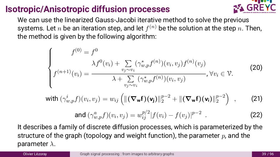
method to solve the previous systems. Let n be an iteration step, and let f(n) be the solution at the step n. Then, the method is given by the following algorithm: f(0) = f0 f(n+1)(vi) = λf0(vi) + vj∼vi (γ∗ w,p f(n))(vi, vj)f(n)(vj) λ + vj∼vi (γ∗ w,p f(n))(vi, vj) , ∀vi ∈ V. (20) with (γi w,p f)(vi, vj) = wij ∥(∇wf)(vj )∥p−2 2 + ∥(∇wf)(vi )∥p−2 2 , (21) and (γa w,p f)(vi, vj) = wp/2 ij |f(vi) − f(vj)|p−2 . (22) It describes a family of discrete diffusion processes, which is parameterized by the structure of the graph (topology and weight function), the parameter p, and the parameter λ. Olivier L´ ezoray Graph signal processing : from images to arbitrary graphs 39 / 96
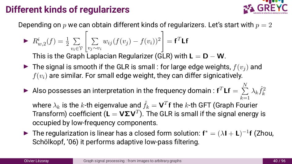
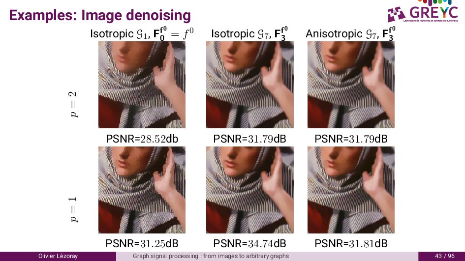
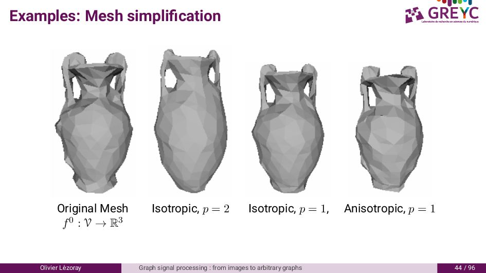
different kinds of regularizers. Let’s start with p = 2 ▶ Ri w,2 (f) = 1 2 vi∈V vj∼vi wij(f(vj) − f(vi))2 = fT Lf This is the Graph Laplacian Regularizer (GLR) with L = D − W. ▶ The signal is smooth if the GLR is small : for large edge weights, f(vj) and f(vi) are similar. For small edge weight, they can differ signicatively. ▶ Also possesses an interpretation in the frequency domain : fT Lf = N k=1 λk ˆ f2 k where λk is the k-th eigenvalue and ˆ fk = VT f the k-th GFT (Graph Fourier Transform) coefficient (L = VΣVT ). The GLR is small if the signal energy is occupied by low-frequency components. ▶ The regularization is linear has a closed form solution: f∗ = (λI + L)−1f (Zhou, Sch¨ olkopf, ’06) it performs adaptive low-pass filtering. Olivier L´ ezoray Graph signal processing : from images to arbitrary graphs 40 / 96
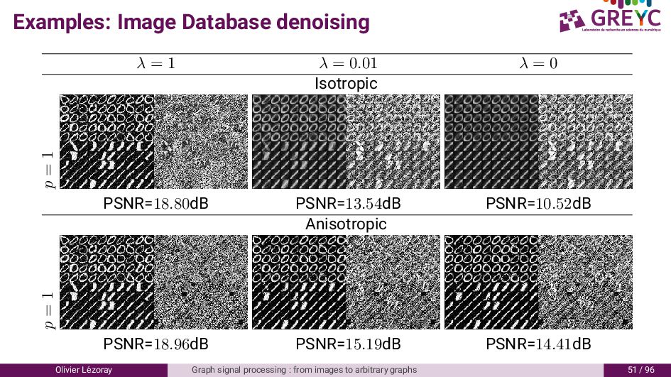
Ri w,1 (f) = vi∈V vj∼vi wij(f(vj) − f(vi))2 1 2 Called the isotropic Graph Total Variation (GTV) ▶ Ra w,1 (f) = vi∈V vj∼vi w1/2 ij |f(vj) − f(vi)| Called the anisotropic Graph Total Variation (GTV) ▶ The GTV is a stronger piecewise smooth prior than the GLR ▶ No closed form-solution as the GTV is non-differentiable ▶ Can be solved more efficiently than with the iterative Gauss-Jacobi process with primal dual algorithms (Chambolle-Pock, ADMM) or the Cut-Pursuit (to be presented) Note : In the GLR and GTV, the graph weights are fixed. There exists other priors where the weights are updated during the minimization (from works of Gene Cheung), called Reweighted GLR and GTV. Olivier L´ ezoray Graph signal processing : from images to arbitrary graphs 41 / 96
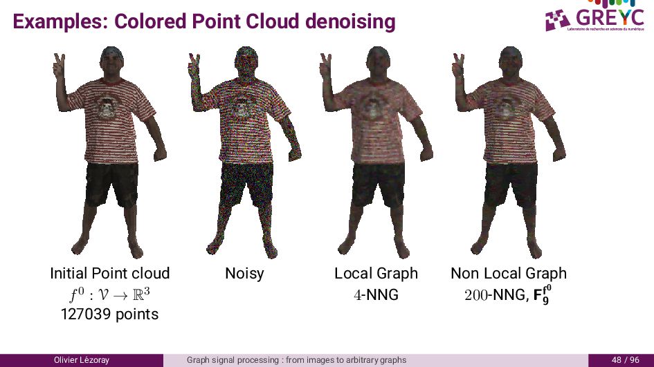
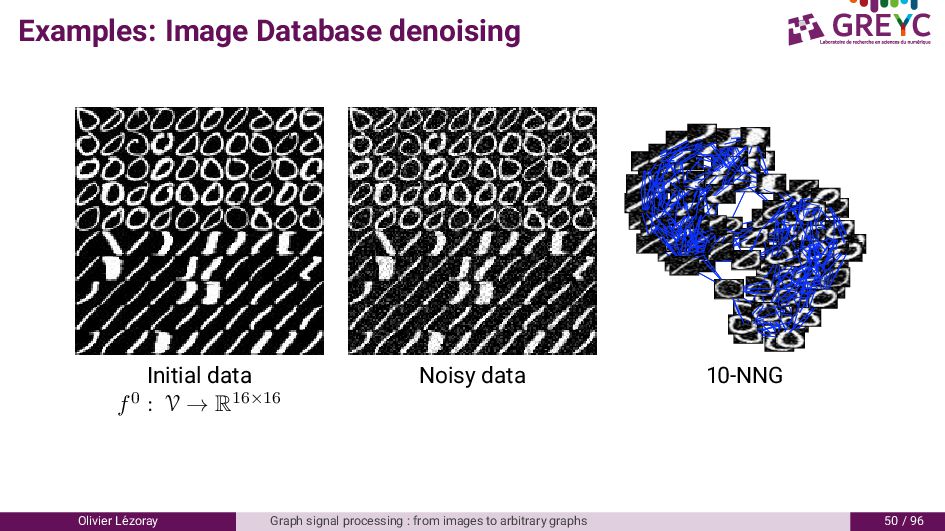
Graph Non Local Graph f0 : V → R3 4-NNG 200-NNG, Ff0 9 127039 points Olivier L´ ezoray Graph signal processing : from images to arbitrary graphs 48 / 96
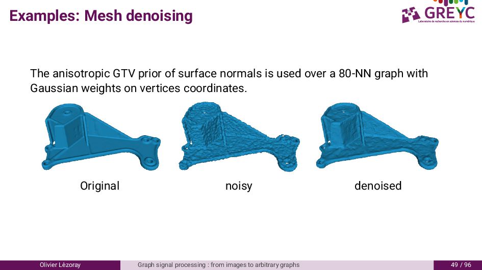
is used over a 80-NN graph with Gaussian weights on vertices coordinates. Original noisy denoised Olivier L´ ezoray Graph signal processing : from images to arbitrary graphs 49 / 96
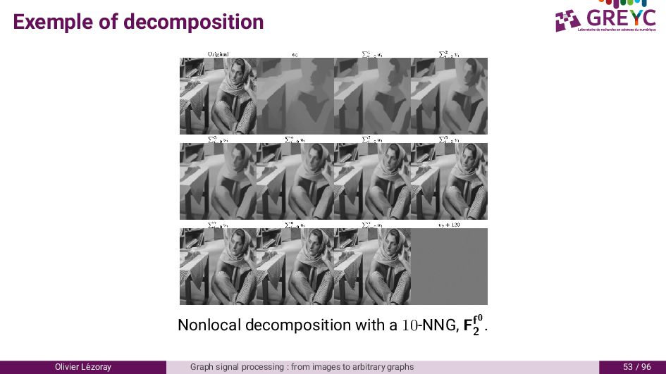
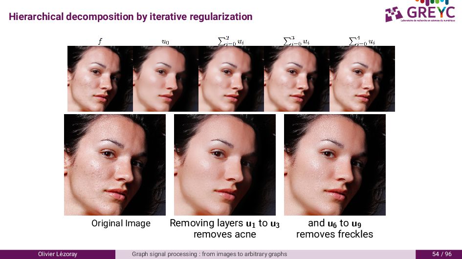
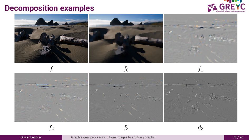
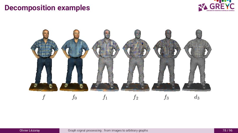
decomposed into a base layer and several detail layers capturing each a given level of detail : f = l−2 i=0 fi + dl−1 ▶ Each layer is obtained by fi = GTVR(di1 ), d−1 = f, and di = di−1 − fi ▶ The sequence of scales is decreaseing λ0 < λ1 < · · · < λl−2 ▶ The signal can be reconstructed from the hierarchical decomposition with linear manipulation of the layers ˆ f(vk) = f0(vk) + l−1 i=1 αifi(vk) with fl−1 = dl−1 ▶ Each layer is boosted is αi > 1. ▶ This is an extension of a hierarchical framework that was proposed by (Tadmor, Nezzar, Vese, ’04) to graph signals on arbitrary graphs Olivier L´ ezoray Graph signal processing : from images to arbitrary graphs 52 / 96
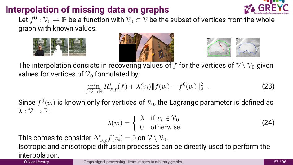
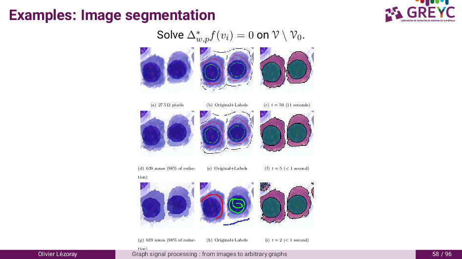
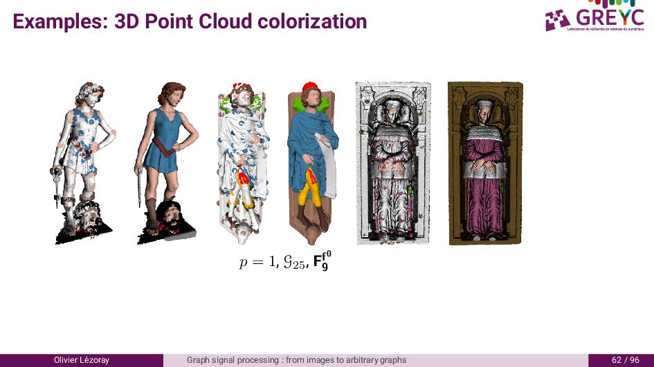
→ R be a function with V0 ⊂ V be the subset of vertices from the whole graph with known values. The interpolation consists in recovering values of f for the vertices of V \ V0 given values for vertices of V0 formulated by: min f:V→R R∗ w,p (f) + λ(vi)∥f(vi) − f0(vi)∥2 2 . (23) Since f0(vi) is known only for vertices of V0, the Lagrange parameter is defined as λ : V → R: λ(vi) = λ if vi ∈ V0 0 otherwise. (24) This comes to consider ∆∗ w,p f(vi) = 0 on V \ V0. Isotropic and anisotropic diffusion processes can be directly used to perform the interpolation. Olivier L´ ezoray Graph signal processing : from images to arbitrary graphs 57 / 96
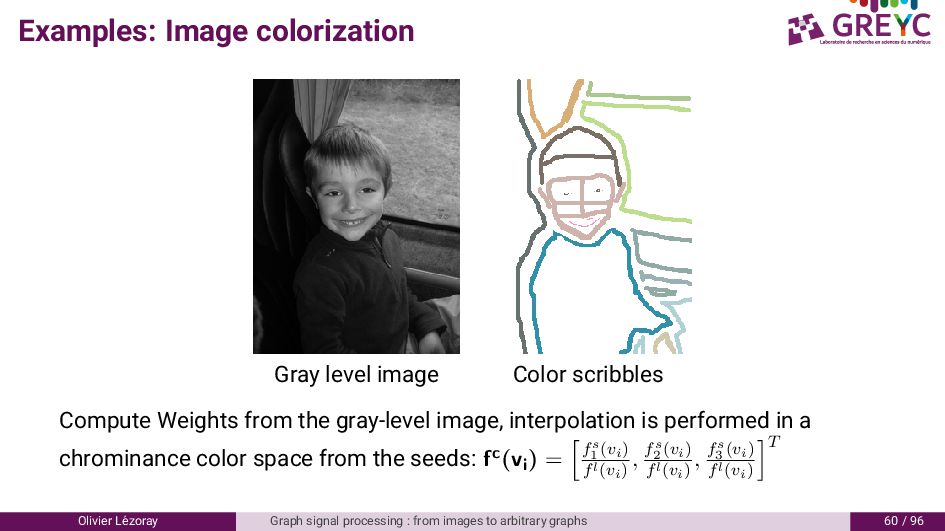
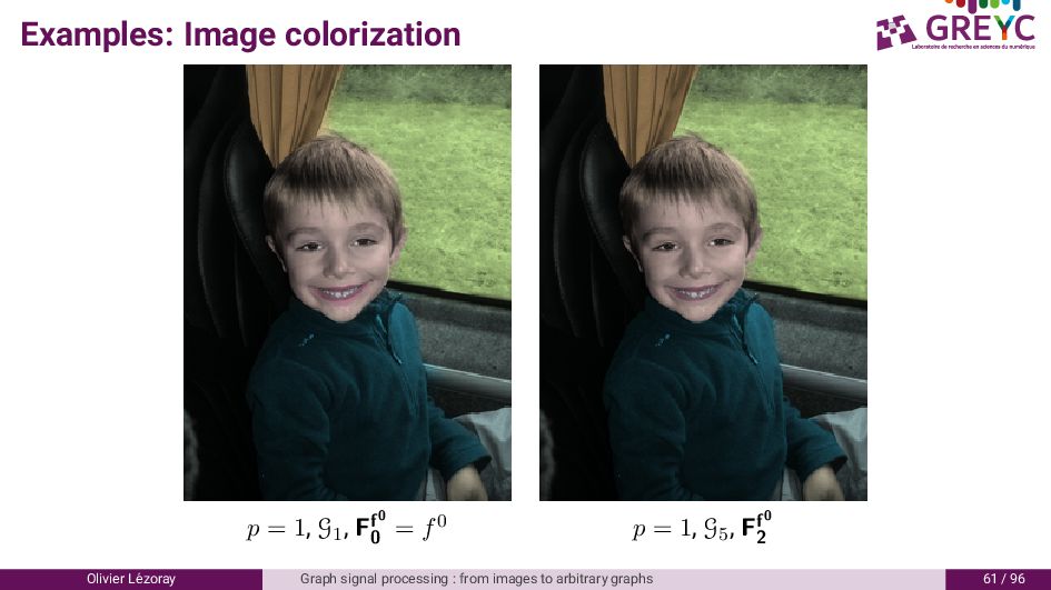
from the gray-level image, interpolation is performed in a chrominance color space from the seeds: fc(vi ) = fs 1 (vi ) fl(vi ) , fs 2 (vi ) fl(vi ) , fs 3 (vi ) fl(vi ) T Olivier L´ ezoray Graph signal processing : from images to arbitrary graphs 60 / 96
4. Graph signal p-Laplacian regularization 5. Mathematical Morphology 6. From continuous MM to Active contours on graphs Olivier L´ ezoray Graph signal processing : from images to arbitrary graphs 63 / 96
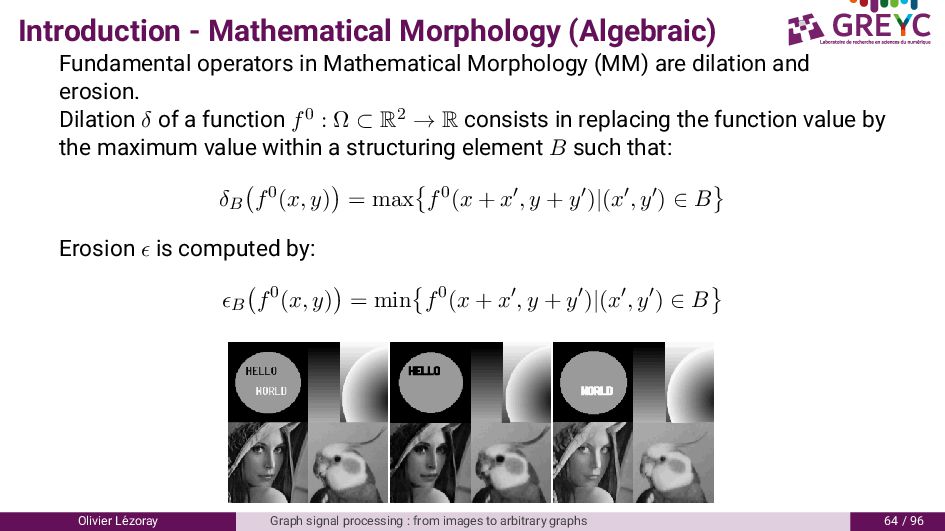
(MM) are dilation and erosion. Dilation δ of a function f0 : Ω ⊂ R2 → R consists in replacing the function value by the maximum value within a structuring element B such that: δB f0(x, y) = max f0(x + x′, y + y′)|(x′, y′) ∈ B Erosion ϵ is computed by: ϵB f0(x, y) = min f0(x + x′, y + y′)|(x′, y′) ∈ B Olivier L´ ezoray Graph signal processing : from images to arbitrary graphs 64 / 96
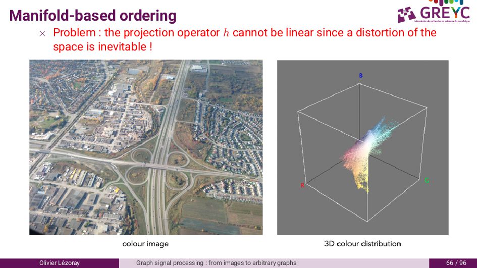
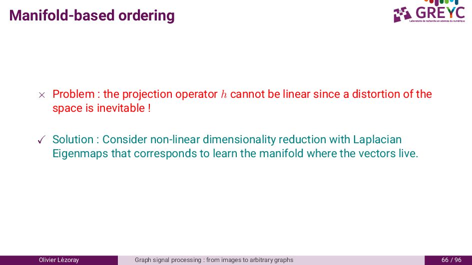
within vectors: a complete lattice (T , ≤) ▶ MM is problematic for multivariate data since there is no natural ordering for vectors ▶ The framework of h-orderings can be considered for that : construct a mapping h from T to L where L is a complete lattice equipped with the conditional total ordering h : T → L and v → h(v), ∀(vi, vj) ∈ T × T vi ≤h vj ⇔ h(vi) ≤ h(vj) . ▶ ≤h denotes such an h-ordering, it is a dimensionality reduction operation h : Rn → Rp with p < n. ▶ Advantage : the learned lattice depends of the signal content and is more adaptive. Olivier L´ ezoray Graph signal processing : from images to arbitrary graphs 65 / 96
be linear since a distortion of the space is inevitable ! ✓ Solution : Consider non-linear dimensionality reduction with Laplacian Eigenmaps that corresponds to learn the manifold where the vectors live. Olivier L´ ezoray Graph signal processing : from images to arbitrary graphs 66 / 96
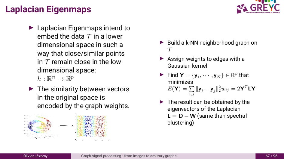
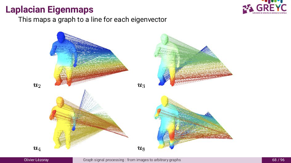
T in a lower dimensional space in such a way that close/similar points in T remain close in the low dimensional space: h : Rn → Rp ▶ The similarity between vectors in the original space is encoded by the graph weights. ▶ Build a k-NN neighborhood graph on T ▶ Assign weights to edges with a Gaussian kernel ▶ Find Y = {y1 , · · · , yN } ∈ Rp that minimizes E(Y) = i,j ∥yi − yj ∥2 2 wij = 2YT LY ▶ The result can be obtained by the eigenvectors of the Laplacian L = D − W (same than spectral clustering) Olivier L´ ezoray Graph signal processing : from images to arbitrary graphs 67 / 96
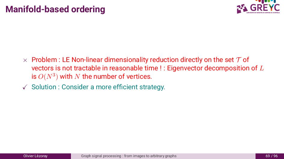
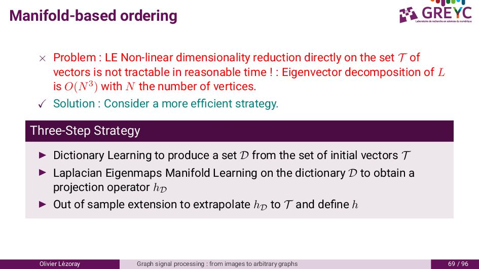
on the set T of vectors is not tractable in reasonable time ! : Eigenvector decomposition of L is O(N3) with N the number of vertices. Olivier L´ ezoray Graph signal processing : from images to arbitrary graphs 69 / 96
on the set T of vectors is not tractable in reasonable time ! : Eigenvector decomposition of L is O(N3) with N the number of vertices. ✓ Solution : Consider a more efficient strategy. Olivier L´ ezoray Graph signal processing : from images to arbitrary graphs 69 / 96
on the set T of vectors is not tractable in reasonable time ! : Eigenvector decomposition of L is O(N3) with N the number of vertices. ✓ Solution : Consider a more efficient strategy. Three-Step Strategy ▶ Dictionary Learning to produce a set D from the set of initial vectors T ▶ Laplacian Eigenmaps Manifold Learning on the dictionary D to obtain a projection operator hD ▶ Out of sample extension to extrapolate hD to T and define h Olivier L´ ezoray Graph signal processing : from images to arbitrary graphs 69 / 96
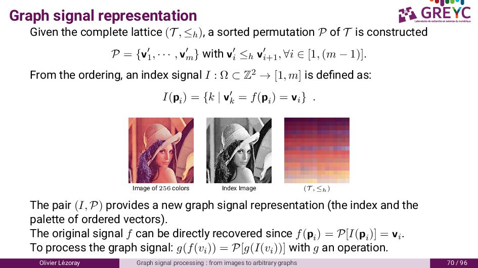
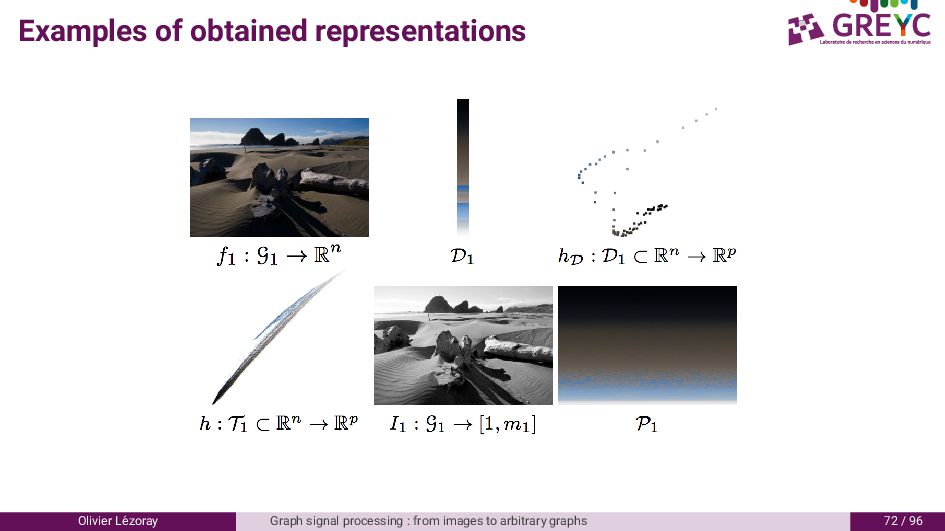
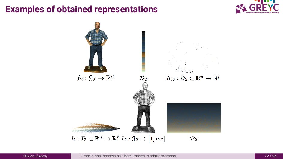
a sorted permutation P of T is constructed P = {v′ 1 , · · · , v′ m } with v′ i ≤h v′ i+1 , ∀i ∈ [1, (m − 1)]. From the ordering, an index signal I : Ω ⊂ Z2 → [1, m] is defined as: I(pi ) = {k | v′ k = f(pi ) = vi } . Image of 256 colors Index Image (T , ≤h) The pair (I, P) provides a new graph signal representation (the index and the palette of ordered vectors). The original signal f can be directly recovered since f(pi ) = P[I(pi )] = vi. To process the graph signal: g(f(vi)) = P[g(I(vi))] with g an operation. Olivier L´ ezoray Graph signal processing : from images to arbitrary graphs 70 / 96
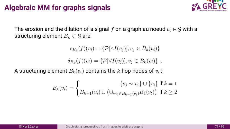
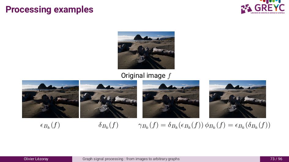
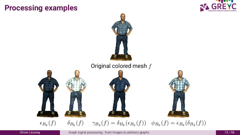
of a signal f on a graph au noeud vi ∈ G with a structuring element Bk ⊂ G are: ϵBk (f)(vi) = {P[∧I(vj)], vj ∈ Bk(vi)} δBk (f)(vi) = {P[∨I(vj)], vj ∈ Bk(vi)} . A structuring element Bk(vi) contains the k-hop nodes of vi : Bk(vi) = {vj ∼ vi } ∪ {vi } if k = 1 Bk−1(vi) ∪ ∪∀vl∈Bk−1 (vi ) B1(vl) if k ≥ 2 Olivier L´ ezoray Graph signal processing : from images to arbitrary graphs 71 / 96
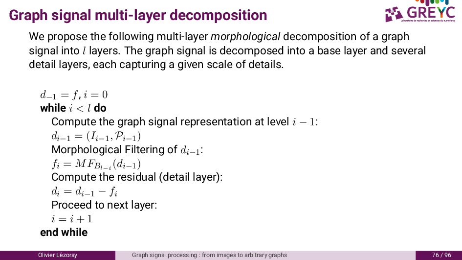
decomposition of a graph signal into l layers. The graph signal is decomposed into a base layer and several detail layers, each capturing a given scale of details. d−1 = f, i = 0 while i < l do Compute the graph signal representation at level i − 1: di−1 = (Ii−1, Pi−1) Morphological Filtering of di−1: fi = MFBl−i (di−1) Compute the residual (detail layer): di = di−1 − fi Proceed to next layer: i = i + 1 end while Olivier L´ ezoray Graph signal processing : from images to arbitrary graphs 76 / 96
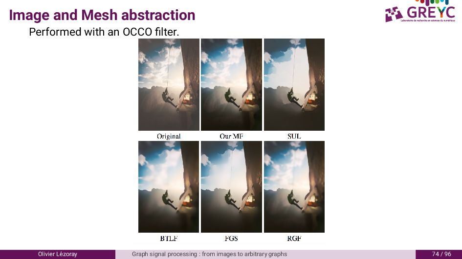
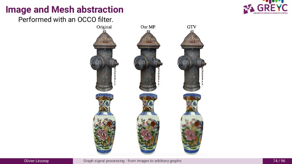
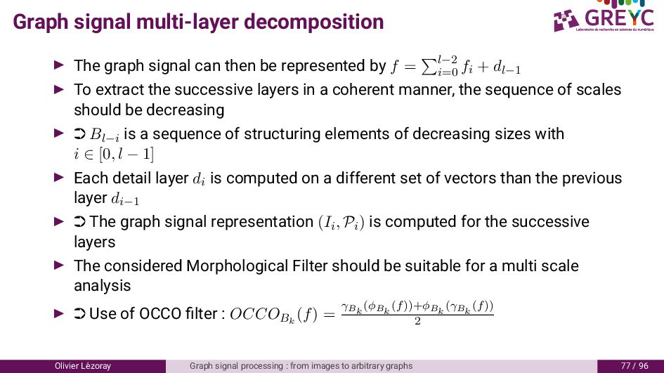
be represented by f = l−2 i=0 fi + dl−1 ▶ To extract the successive layers in a coherent manner, the sequence of scales should be decreasing ▶ ➲ Bl−i is a sequence of structuring elements of decreasing sizes with i ∈ [0, l − 1] ▶ Each detail layer di is computed on a different set of vectors than the previous layer di−1 ▶ ➲ The graph signal representation (Ii, Pi) is computed for the successive layers ▶ The considered Morphological Filter should be suitable for a multi scale analysis ▶ ➲ Use of OCCO filter : OCCOBk (f) = γBk (ϕBk (f))+ϕBk (γBk (f)) 2 Olivier L´ ezoray Graph signal processing : from images to arbitrary graphs 77 / 96
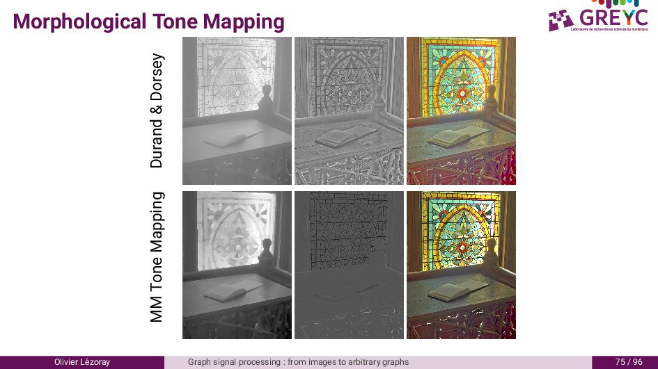
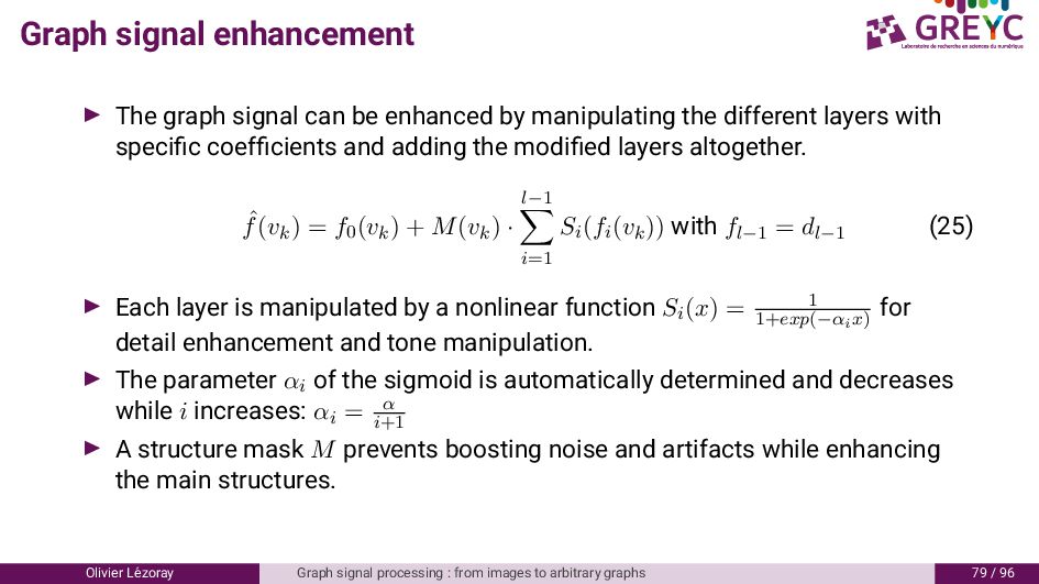
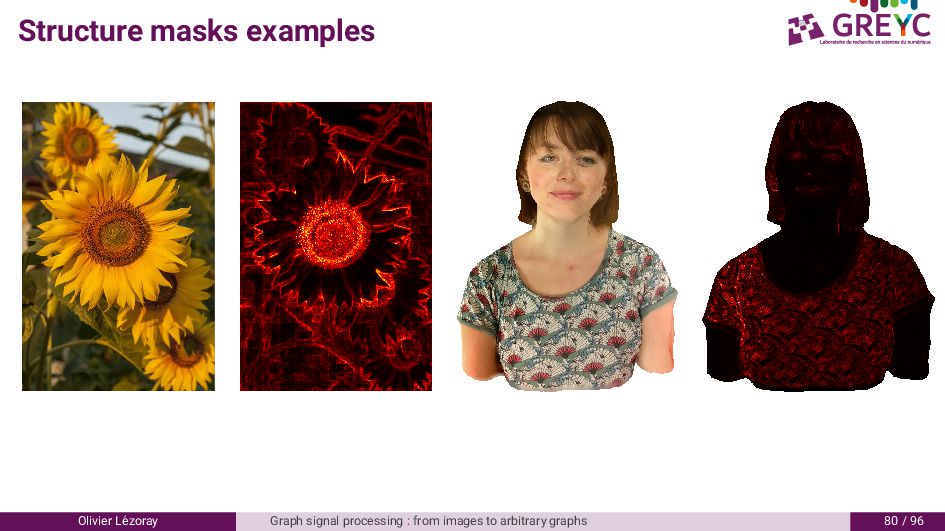
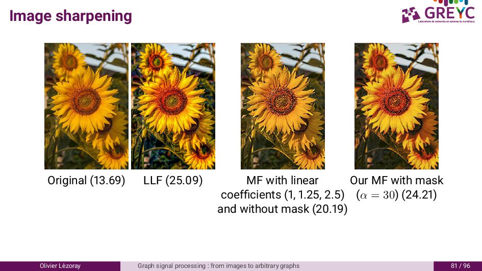
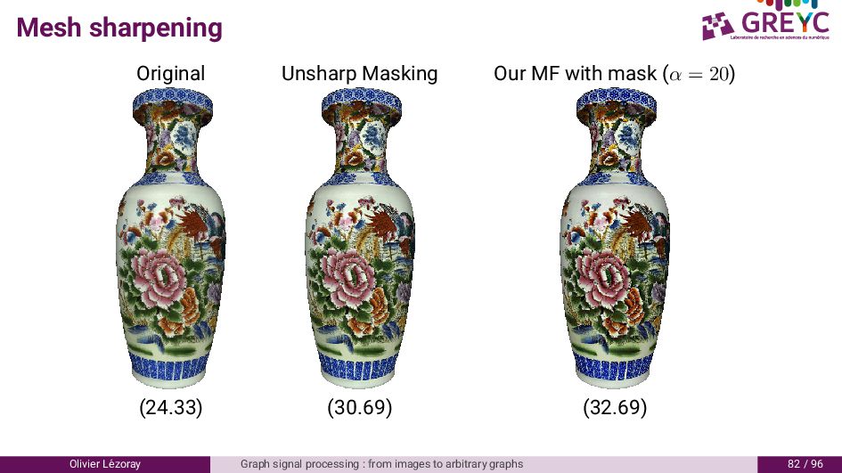
by manipulating the different layers with specific coefficients and adding the modified layers altogether. ˆ f(vk) = f0(vk) + M(vk) · l−1 i=1 Si(fi(vk)) with fl−1 = dl−1 (25) ▶ Each layer is manipulated by a nonlinear function Si(x) = 1 1+exp(−αi x) for detail enhancement and tone manipulation. ▶ The parameter αi of the sigmoid is automatically determined and decreases while i increases: αi = α i+1 ▶ A structure mask M prevents boosting noise and artifacts while enhancing the main structures. Olivier L´ ezoray Graph signal processing : from images to arbitrary graphs 79 / 96
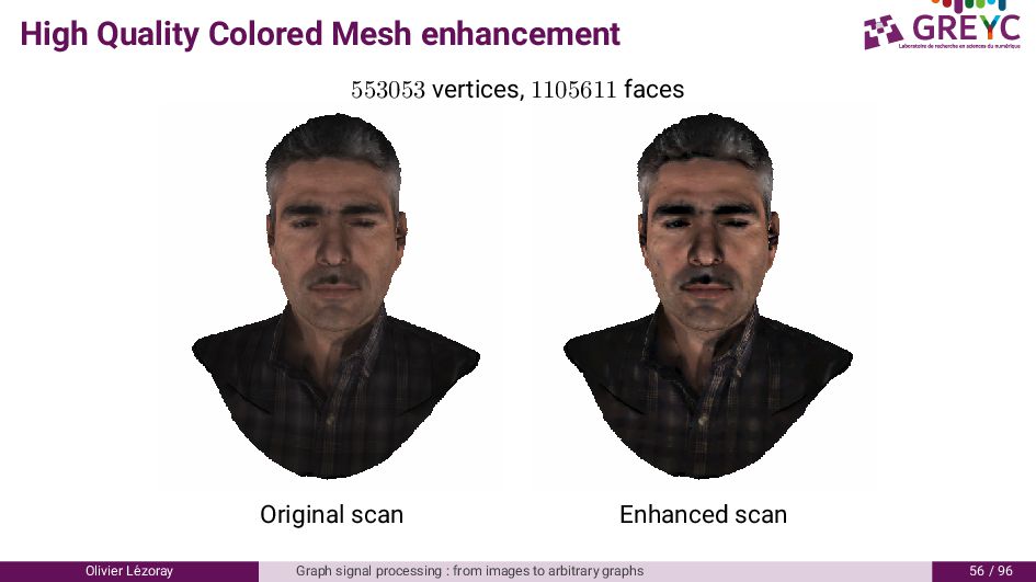
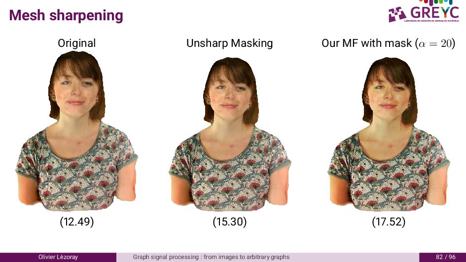
MF with mask coefficients (1, 1.25, 2.5) (α = 30) (24.21) and without mask (20.19) Olivier L´ ezoray Graph signal processing : from images to arbitrary graphs 81 / 96
4. Graph signal p-Laplacian regularization 5. Mathematical Morphology 6. From continuous MM to Active contours on graphs Olivier L´ ezoray Graph signal processing : from images to arbitrary graphs 83 / 96
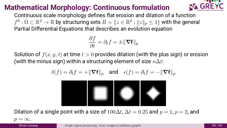
and dilation of a function f0 : Ω ⊂ R2 → R by structuring sets B = {z ∈ R2 : ∥z∥p ≤ 1} with the general Partial Differential Equations that describes an evolution equation ∂f ∂t = ∂tf = ±∥∇f∥p Solution of f(x, y, t) at time t > 0 provides dilation (with the plus sign) or erosion (with the minus sign) within a structuring element of size n∆t: δ(f) = ∂tf = +∥∇f∥p and ϵ(f) = ∂tf = −∥∇f∥p Dilation of a single point with a size of 100∆t, ∆t = 0.25 and p = 1, p = 2, and p = ∞. Olivier L´ ezoray Graph signal processing : from images to arbitrary graphs 84 / 96
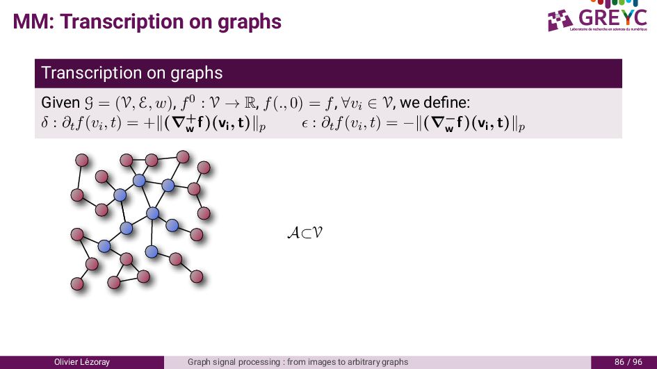
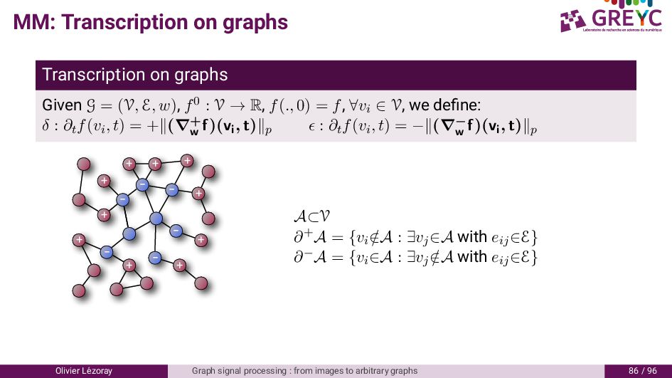
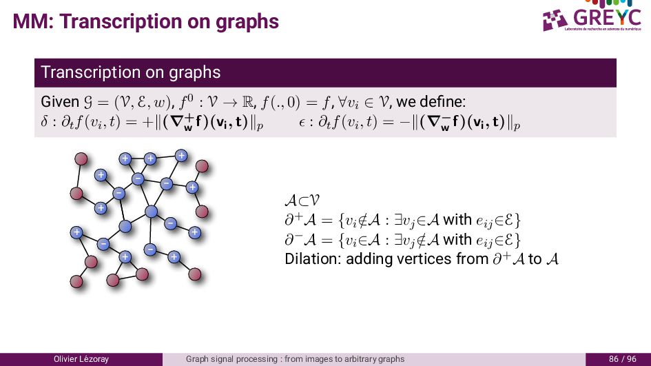
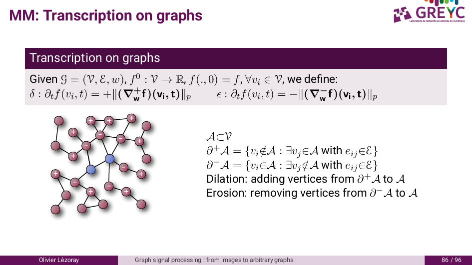
difference operators (weighted directional operators): (d+ w f)(vi, vj)=w(vi, vj)1/2 max f(vi), f(vj) −f(vi) and (d− w f)(vi, vj)=w(vi, vj)1/2 f(vi)− min f(vi), f(vj) , (26) with the following properties (always positive) (d+ w f)(vi, vj)= max 0, (dwf)(vi, vj) (d− w f)(vi, vj)= − min 0, (dwf)(vi, vj) with the associated internal and external gradients: (∇± w f)(vi ) = [(d± w f)(vi, vj) : ∀vj ∈ V]T . Olivier L´ ezoray Graph signal processing : from images to arbitrary graphs 85 / 96
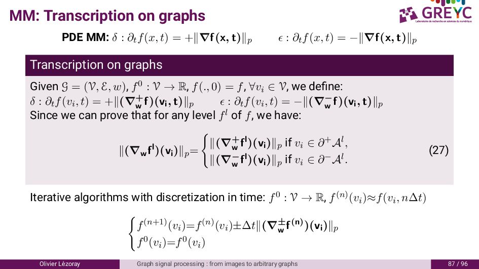
= +∥∇f(x, t)∥p ϵ : ∂tf(x, t) = −∥∇f(x, t)∥p Transcription on graphs Given G = (V, E, w), f0 : V → R, f(., 0) = f, ∀vi ∈ V, we define: δ : ∂tf(vi, t) = +∥(∇+ w f)(vi, t)∥p ϵ : ∂tf(vi, t) = −∥(∇− w f)(vi, t)∥p Since we can prove that for any level fl of f, we have: ∥(∇wfl)(vi )∥p= ∥(∇+ w fl)(vi )∥p if vi ∈ ∂+Al, ∥(∇− w fl)(vi )∥p if vi ∈ ∂−Al. (27) Iterative algorithms with discretization in time: f0 : V → R, f(n)(vi)≈f(vi, n∆t) f(n+1)(vi)=f(n)(vi)±∆t∥(∇± w f(n))(vi )∥p f0(vi)=f0(vi) Olivier L´ ezoray Graph signal processing : from images to arbitrary graphs 87 / 96
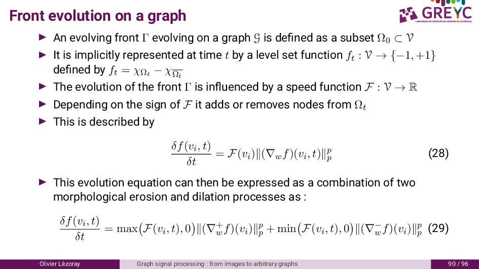
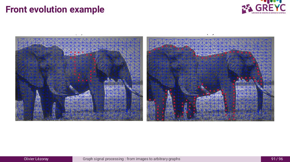
evolving on a graph G is defined as a subset Ω0 ⊂ V ▶ It is implicitly represented at time t by a level set function ft : V → {−1, +1} defined by ft = χΩt − χ Ωt ▶ The evolution of the front Γ is influenced by a speed function F : V → R ▶ Depending on the sign of F it adds or removes nodes from Ωt ▶ This is described by δf(vi, t) δt = F(vi)∥(∇wf)(vi, t)∥p p (28) ▶ This evolution equation can then be expressed as a combination of two morphological erosion and dilation processes as : δf(vi, t) δt = max F(vi, t), 0 ∥(∇+ w f)(vi)∥p p + min F(vi, t), 0 ∥(∇− w f)(vi)∥p p (29) Olivier L´ ezoray Graph signal processing : from images to arbitrary graphs 90 / 96
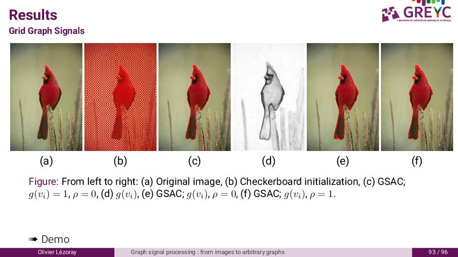
and without edges actives contours Our adaptation ▶ Given f a level set function ft : V → {−1, +1} for inside/outside of the evolving propagating front, the solution is obtained by ft+1(vi ) = ft(vi ) + ∆tδf(vi,t) δt ▶ We express front propagation on graphs as δf(vi,t) δt = F(vi , t)∥(∇w f)(vi , t)∥p p with F(vi , t) a speed function ▶ We propose a front propagation function that solves the considered active contours with discrete calculus: F(vi , t) = νg(vi ) + µg(vi )(κw f)(vi , t) − λ1 d vi d2(Ff0 ρ (vi ), Fc1 ρ ) + λ2 d vi d2(Ff0 ρ (vi ), Fc2 ρ ) ▶ We consider local patches Ff0 ρ (vj ) on a ρ-hop subgraph to represent the regions (instead of vertex-based signal average) ▶ The potential function g(vi ) differentiates the most salient structures of a graph using patches comparison: as in MM enhancement Olivier L´ ezoray Graph signal processing : from images to arbitrary graphs 92 / 96
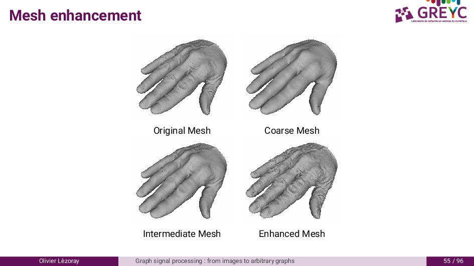
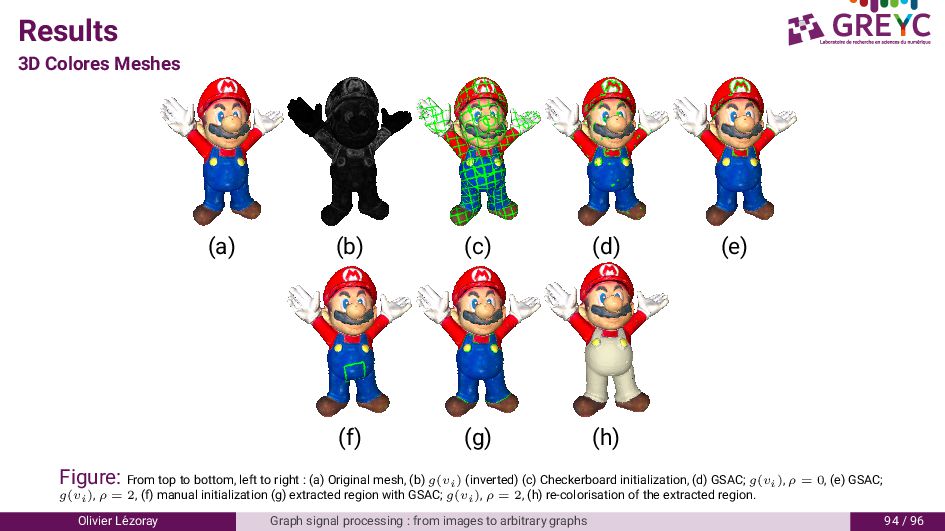
(g) (h) Figure: From top to bottom, left to right : (a) Original mesh, (b) g(vi) (inverted) (c) Checkerboard initialization, (d) GSAC; g(vi), ρ = 0, (e) GSAC; g(vi), ρ = 2, (f) manual initialization (g) extracted region with GSAC; g(vi), ρ = 2, (h) re-colorisation of the extracted region. Olivier L´ ezoray Graph signal processing : from images to arbitrary graphs 94 / 96
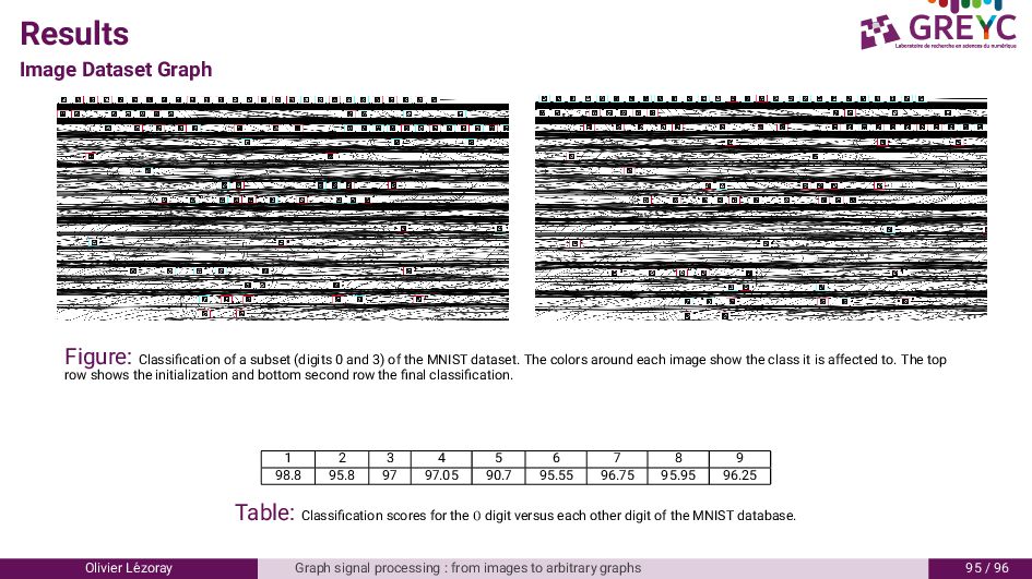
0 and 3) of the MNIST dataset. The colors around each image show the class it is affected to. The top row shows the initialization and bottom second row the final classification. 1 2 3 4 5 6 7 8 9 98.8 95.8 97 97.05 90.7 95.55 96.75 95.95 96.25 Table: Classification scores for the 0 digit versus each other digit of the MNIST database. Olivier L´ ezoray Graph signal processing : from images to arbitrary graphs 95 / 96
![The end [thank you] Any Questions ? [email protected] https://lezoray.users.greyc.fr Olivier](https://files.speakerdeck.com/presentations/985afbdc04f44dffabf904fe7d767b73/slide_121.jpg)