Seminar at LEOST-UGE, Lille

Transcript

1. VARIATIONAL, MORPHOLOGICAL AND NEURAL APPROACHES TO GRAPH SIGNAL PROCESSING Olivier L´ ezoray Normandie Univ, UNICAEN, ENSICAEN, CNRS, GREYC, Caen, FRANCE olivier.lezoray@unicaen.fr https://lezoray.users.greyc.fr
2. Normandy ? Olivier L´ ezoray Variational, morphological and neural approaches to graph signal processing / 6
3. UNICAEN / GREYC Lab Founded in , by the king of England Henri VI, when the region was English (third English university, after Oxford and Cambridge). Completely destroyed in and rebuilt in (the phoenix rising from its ashes). UMR CNRS, largest lab in Normandy ( persons), 6 research teams on digital sciences. Olivier L´ ezoray Variational, morphological and neural approaches to graph signal processing / 6
4. . Introduction . Notations . p-Laplacian adaptive filtering . Active contours on graphs . Morphological decomposition of graphs signals 6. Morphological segmentation of graph signals . Hand gesture recognition Olivier L´ ezoray Variational, morphological and neural approaches to graph signal processing / 6
5. . Introduction . Notations . p-Laplacian adaptive filtering . Active contours on graphs . Morphological decomposition of graphs signals 6. Morphological segmentation of graph signals . Hand gesture recognition Olivier L´ ezoray Variational, morphological and neural approaches to graph signal processing / 6
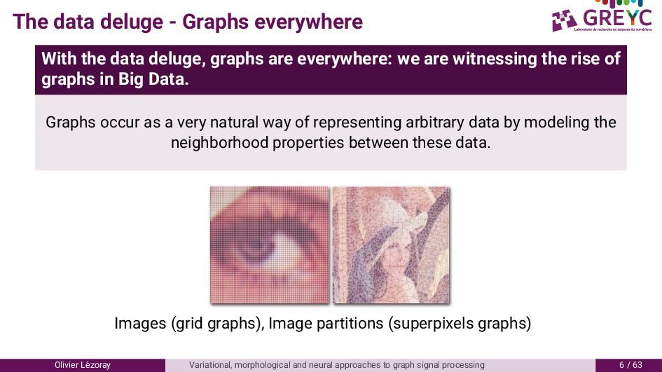
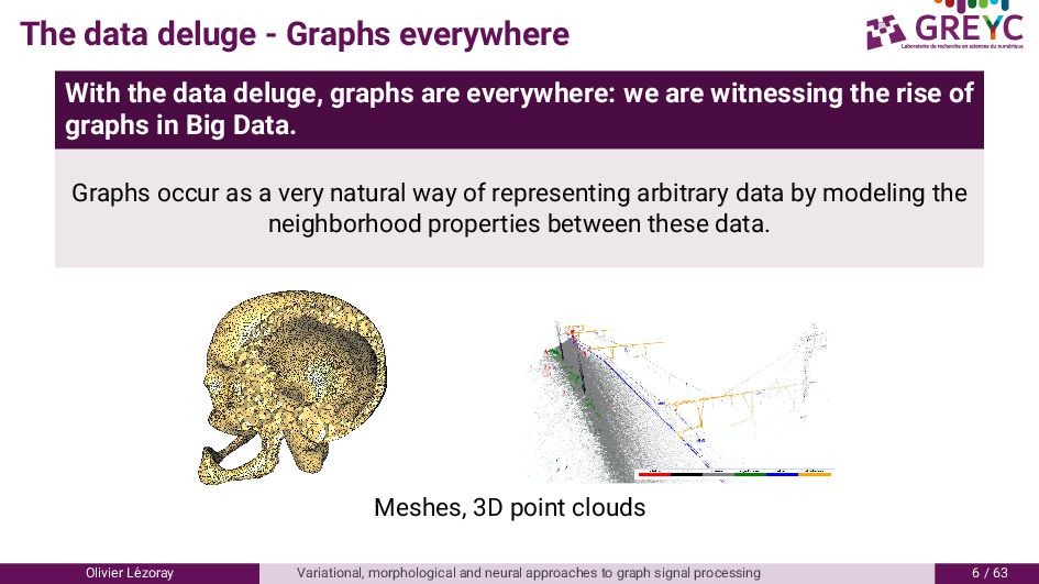
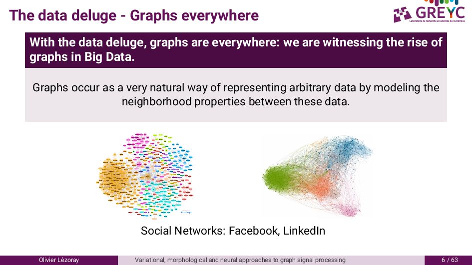
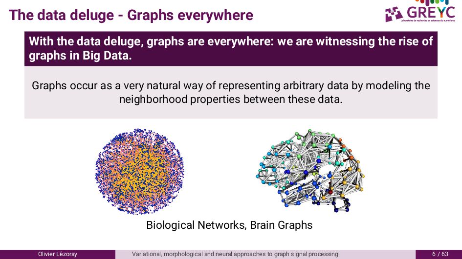
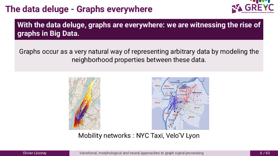
6. The data deluge - Graphs everywhere With the data deluge, graphs are everywhere: we are witnessing the rise of graphs in Big Data. Graphs occur as a very natural way of representing arbitrary data by modeling the neighborhood properties between these data. Olivier L´ ezoray Variational, morphological and neural approaches to graph signal processing 6 / 6
7. The data deluge - Graphs everywhere With the data deluge, graphs are everywhere: we are witnessing the rise of graphs in Big Data. Graphs occur as a very natural way of representing arbitrary data by modeling the neighborhood properties between these data. Images (grid graphs), Image partitions (superpixels graphs) Olivier L´ ezoray Variational, morphological and neural approaches to graph signal processing 6 / 6
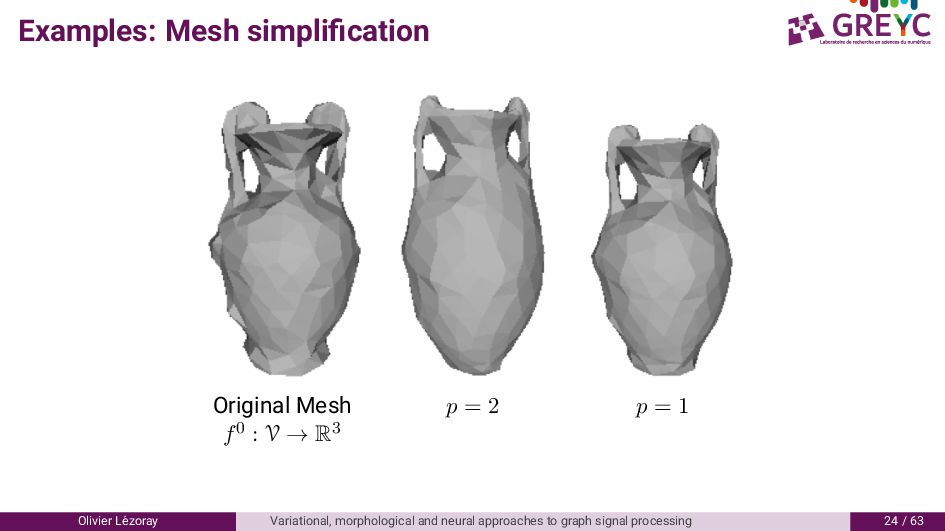
8. The data deluge - Graphs everywhere With the data deluge, graphs are everywhere: we are witnessing the rise of graphs in Big Data. Graphs occur as a very natural way of representing arbitrary data by modeling the neighborhood properties between these data. Meshes, D point clouds Olivier L´ ezoray Variational, morphological and neural approaches to graph signal processing 6 / 6
9. The data deluge - Graphs everywhere With the data deluge, graphs are everywhere: we are witnessing the rise of graphs in Big Data. Graphs occur as a very natural way of representing arbitrary data by modeling the neighborhood properties between these data. Social Networks: Facebook, LinkedIn Olivier L´ ezoray Variational, morphological and neural approaches to graph signal processing 6 / 6
10. The data deluge - Graphs everywhere With the data deluge, graphs are everywhere: we are witnessing the rise of graphs in Big Data. Graphs occur as a very natural way of representing arbitrary data by modeling the neighborhood properties between these data. Biological Networks, Brain Graphs Olivier L´ ezoray Variational, morphological and neural approaches to graph signal processing 6 / 6
11. The data deluge - Graphs everywhere With the data deluge, graphs are everywhere: we are witnessing the rise of graphs in Big Data. Graphs occur as a very natural way of representing arbitrary data by modeling the neighborhood properties between these data. Mobility networks : NYC Taxi, Velo’V Lyon Olivier L´ ezoray Variational, morphological and neural approaches to graph signal processing 6 / 6
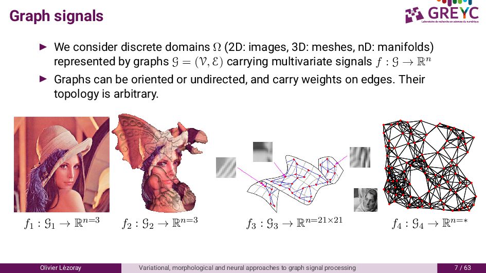
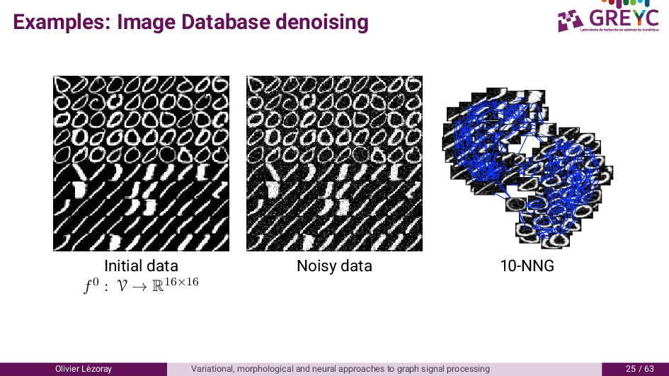
12. Graph signals We consider discrete domains Ω ( D: images, D: meshes, nD: manifolds) represented by graphs G = (V, E) carrying multivariate signals f : G → Rn Graphs can be oriented or undirected, and carry weights on edges. Their topology is arbitrary. f1 : G1 → Rn=3 f2 : G2 → Rn=3 f3 : G3 → Rn=21×21 f4 : G4 → Rn=∗ Olivier L´ ezoray Variational, morphological and neural approaches to graph signal processing / 6
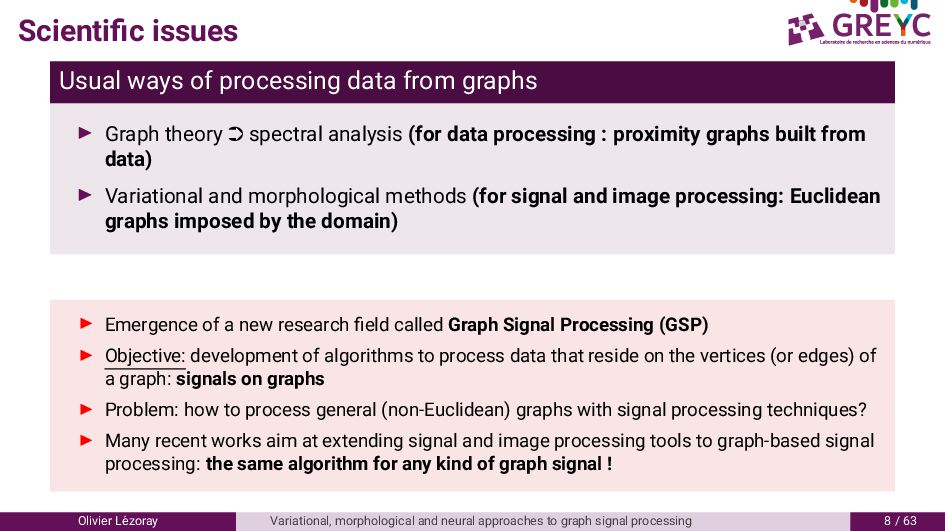
13. Scientific issues Usual ways of processing data from graphs Graph theory · spectral analysis (for data processing : proximity graphs built from data) Variational and morphological methods (for signal and image processing: Euclidean graphs imposed by the domain) Emergence of a new research field called Graph Signal Processing (GSP) Objective: development of algorithms to process data that reside on the vertices (or edges) of a graph: signals on graphs Problem: how to process general (non-Euclidean) graphs with signal processing techniques? Many recent works aim at extending signal and image processing tools to graph-based signal processing: the same algorithm for any kind of graph signal ! Olivier L´ ezoray Variational, morphological and neural approaches to graph signal processing 8 / 6
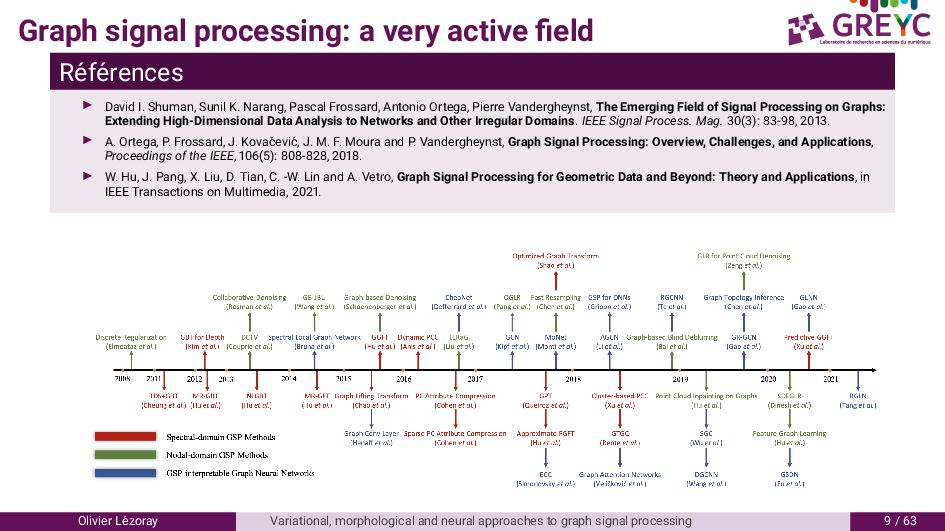
14. Graph signal processing: a very active field R´ ef´ erences David I. Shuman, Sunil K. Narang, Pascal Frossard, Antonio Ortega, Pierre Vandergheynst, The Emerging Field of Signal Processing on Graphs: Extending High-Dimensional Data Analysis to Networks and Other Irregular Domains. IEEE Signal Process. Mag. ( ): 8 - 8, . A. Ortega, P. Frossard, J. Kovaˇ cevi´ c, J. M. F. Moura and P. Vandergheynst, Graph Signal Processing: Overview, Challenges, and Applications, Proceedings of the IEEE, 6( ): 8 8-8 8, 8. W. Hu, J. Pang, X. Liu, D. Tian, C. -W. Lin and A. Vetro, Graph Signal Processing for Geometric Data and Beyond: Theory and Applications, in IEEE Transactions on Multimedia, . Olivier L´ ezoray Variational, morphological and neural approaches to graph signal processing / 6
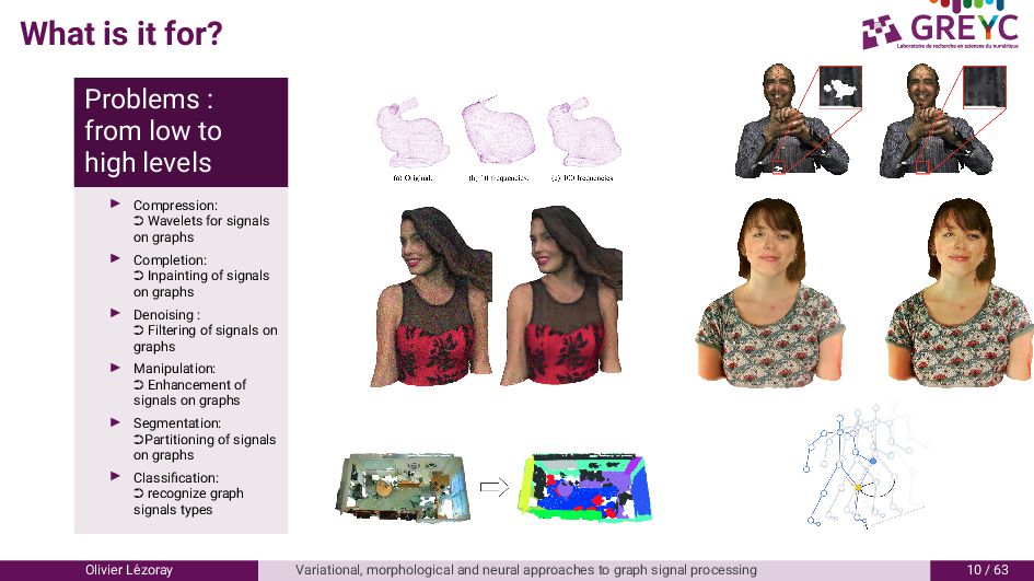
15. What is it for? Problems : from low to high levels Compression: · Wavelets for signals on graphs Completion: · Inpainting of signals on graphs Denoising : · Filtering of signals on graphs Manipulation: · Enhancement of signals on graphs Segmentation: ·Partitioning of signals on graphs Classification: · recognize graph signals types Olivier L´ ezoray Variational, morphological and neural approaches to graph signal processing / 6
16. . Introduction . Notations . p-Laplacian adaptive filtering . Active contours on graphs . Morphological decomposition of graphs signals 6. Morphological segmentation of graph signals . Hand gesture recognition Olivier L´ ezoray Variational, morphological and neural approaches to graph signal processing / 6
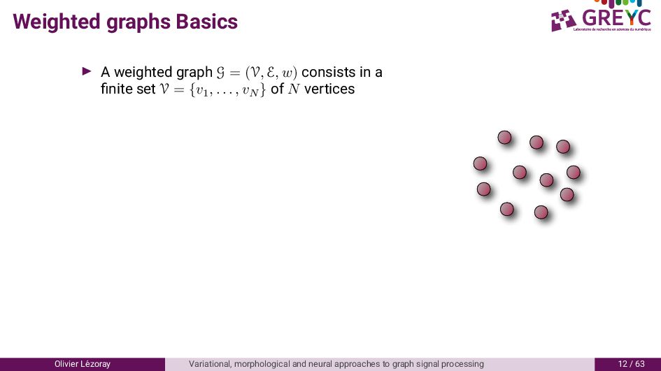
17. Weighted graphs Basics A weighted graph G = (V, E, w) consists in a finite set V = {v1 , . . . , vN } of N vertices Olivier L´ ezoray Variational, morphological and neural approaches to graph signal processing / 6
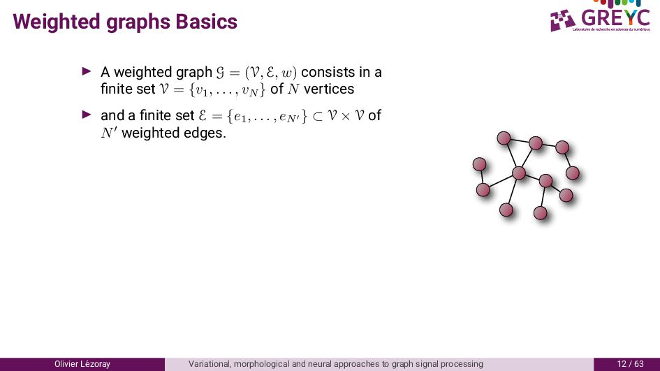
18. Weighted graphs Basics A weighted graph G = (V, E, w) consists in a finite set V = {v1 , . . . , vN } of N vertices and a finite set E = {e1 , . . . , eN } ⊂ V × V of N weighted edges. Olivier L´ ezoray Variational, morphological and neural approaches to graph signal processing / 6
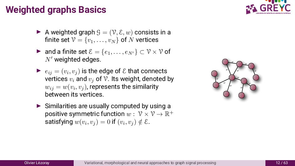
19. Weighted graphs Basics A weighted graph G = (V, E, w) consists in a finite set V = {v1 , . . . , vN } of N vertices and a finite set E = {e1 , . . . , eN } ⊂ V × V of N weighted edges. eij = (vi , vj ) is the edge of E that connects vertices vi and vj of V. Its weight, denoted by wij = w(vi , vj ), represents the similarity between its vertices. Similarities are usually computed by using a positive symmetric function w : V × V → R+ satisfying w(vi , vj ) = 0 if (vi , vj ) / ∈ E. w w w w w w w w w w w Olivier L´ ezoray Variational, morphological and neural approaches to graph signal processing / 6
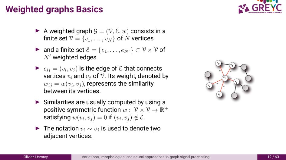
20. Weighted graphs Basics A weighted graph G = (V, E, w) consists in a finite set V = {v1 , . . . , vN } of N vertices and a finite set E = {e1 , . . . , eN } ⊂ V × V of N weighted edges. eij = (vi , vj ) is the edge of E that connects vertices vi and vj of V. Its weight, denoted by wij = w(vi , vj ), represents the similarity between its vertices. Similarities are usually computed by using a positive symmetric function w : V × V → R+ satisfying w(vi , vj ) = 0 if (vi , vj ) / ∈ E. The notation vi ∼ vj is used to denote two adjacent vertices. Olivier L´ ezoray Variational, morphological and neural approaches to graph signal processing / 6
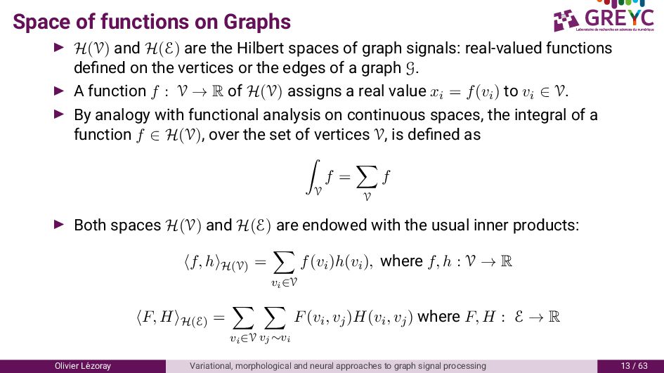
21. Space of functions on Graphs H(V) and H(E) are the Hilbert spaces of graph signals: real-valued functions defined on the vertices or the edges of a graph G. A function f : V → R of H(V) assigns a real value xi = f(vi) to vi ∈ V. By analogy with functional analysis on continuous spaces, the integral of a function f ∈ H(V), over the set of vertices V, is defined as V f = V f Both spaces H(V) and H(E) are endowed with the usual inner products: f, h H(V) = vi∈V f(vi)h(vi), where f, h : V → R F, H H(E) = vi∈V vj∼vi F(vi, vj)H(vi, vj) where F, H : E → R Olivier L´ ezoray Variational, morphological and neural approaches to graph signal processing / 6
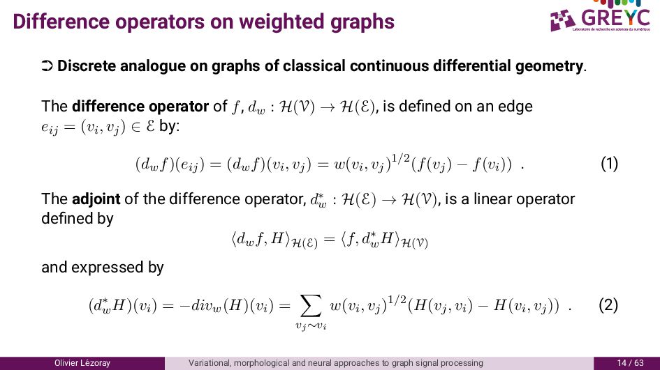
22. Difference operators on weighted graphs · Discrete analogue on graphs of classical continuous differential geometry. The difference operator of f, dw : H(V) → H(E), is defined on an edge eij = (vi, vj) ∈ E by: (dwf)(eij) = (dwf)(vi, vj) = w(vi, vj)1/2(f(vj) − f(vi)) . ( ) The adjoint of the difference operator, d∗ w : H(E) → H(V), is a linear operator defined by dwf, H H(E) = f, d∗ w H H(V) and expressed by (d∗ w H)(vi) = −divw(H)(vi) = vj∼vi w(vi, vj)1/2(H(vj, vi) − H(vi, vj)) . ( ) Olivier L´ ezoray Variational, morphological and neural approaches to graph signal processing / 6
23. Difference operators on weighted graphs The directional derivative (or edge derivative) of f, at a vertex vi ∈ V, along an edge eij = (vi, vj), is defined as ∂f ∂eij vi = ∂vj f(vi) = (dwf)(vi, vj) = w(vi, vj)1/2(f(vj) − f(vi)) Weighted finite difference correspond to forward differences on grid-graph images with w(vi, vj) = 1 h2 with h2 the discretization step: ∂f ∂x (vi) = f(vi + h2) − f(vi) h2 Olivier L´ ezoray Variational, morphological and neural approaches to graph signal processing / 6
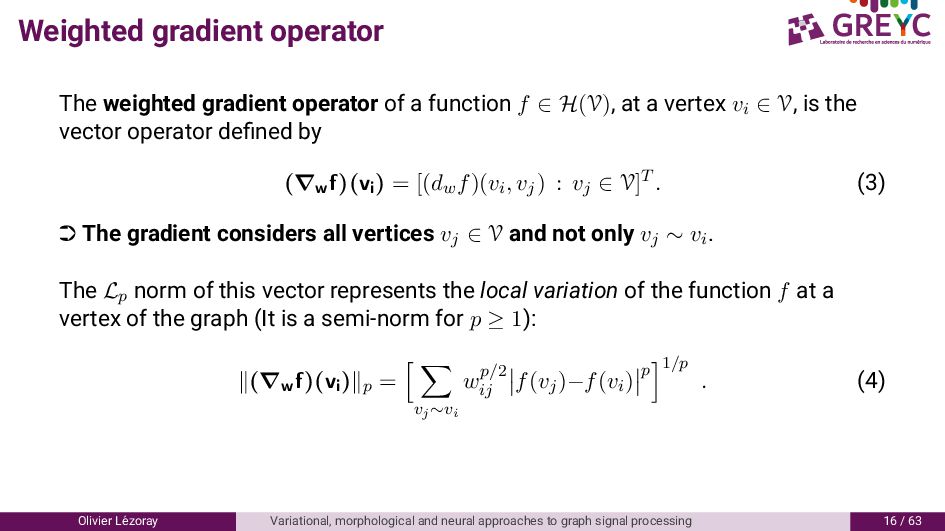
24. Weighted gradient operator The weighted gradient operator of a function f ∈ H(V), at a vertex vi ∈ V, is the vector operator defined by (∇wf)(vi) = [(dwf)(vi, vj) : vj ∈ V]T . ( ) · The gradient considers all vertices vj ∈ V and not only vj ∼ vi . The Lp norm of this vector represents the local variation of the function f at a vertex of the graph (It is a semi-norm for p ≥ 1): (∇wf)(vi) p = vj∼vi wp/2 ij f(vj)−f(vi) p 1/p . ( ) Olivier L´ ezoray Variational, morphological and neural approaches to graph signal processing 6 / 6
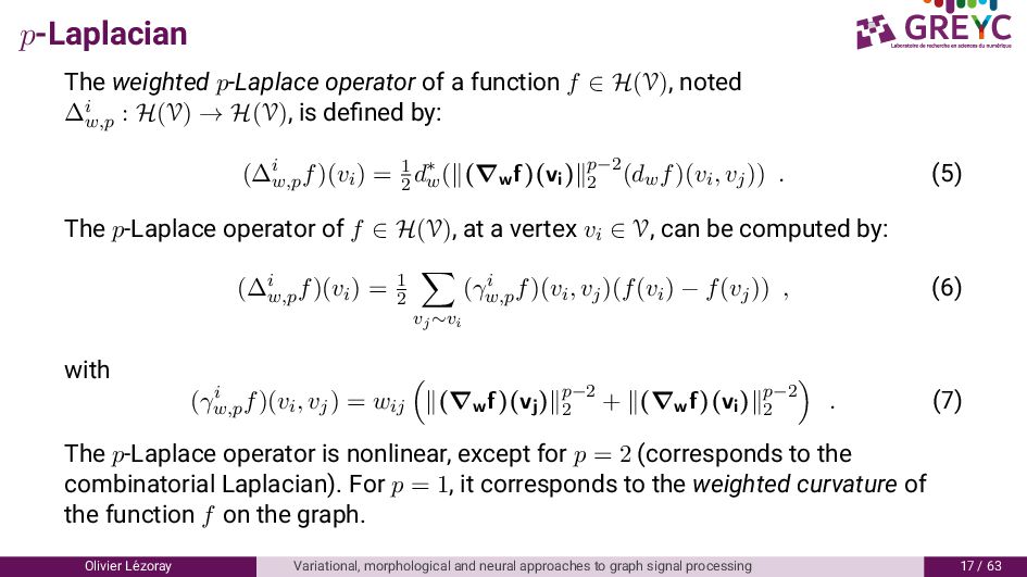
25. p-Laplacian The weighted p-Laplace operator of a function f ∈ H(V), noted ∆i w,p : H(V) → H(V), is defined by: (∆i w,p f)(vi) = 1 2 d∗ w ( (∇wf)(vi) p−2 2 (dwf)(vi, vj)) . ( ) The p-Laplace operator of f ∈ H(V), at a vertex vi ∈ V, can be computed by: (∆i w,p f)(vi) = 1 2 vj∼vi (γi w,p f)(vi, vj)(f(vi) − f(vj)) , (6) with (γi w,p f)(vi, vj) = wij (∇wf)(vj) p−2 2 + (∇wf)(vi) p−2 2 . ( ) The p-Laplace operator is nonlinear, except for p = 2 (corresponds to the combinatorial Laplacian). For p = 1, it corresponds to the weighted curvature of the function f on the graph. Olivier L´ ezoray Variational, morphological and neural approaches to graph signal processing / 6
26. . Introduction . Notations . p-Laplacian adaptive filtering . Active contours on graphs . Morphological decomposition of graphs signals 6. Morphological segmentation of graph signals . Hand gesture recognition Olivier L´ ezoray Variational, morphological and neural approaches to graph signal processing 8 / 6
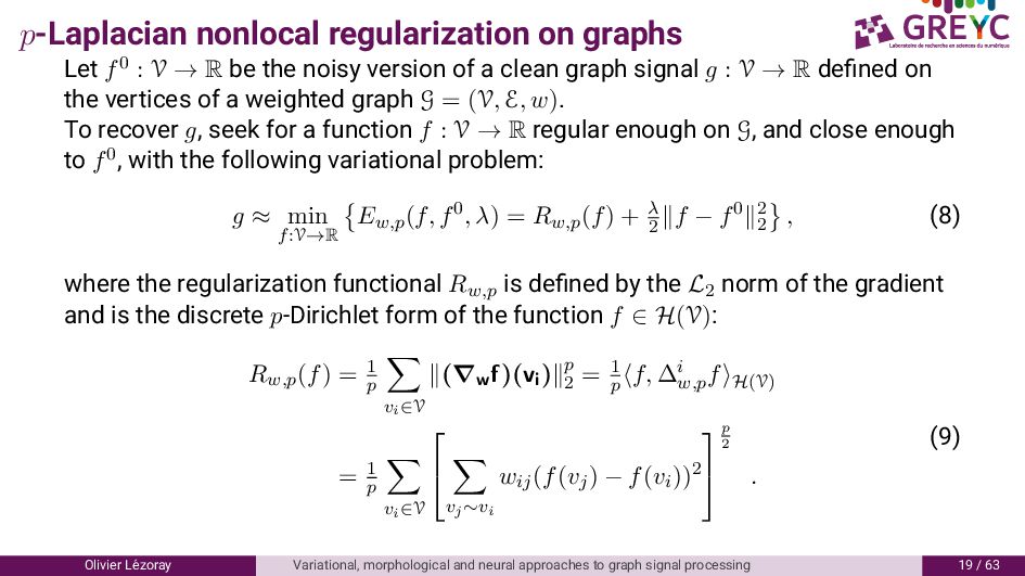
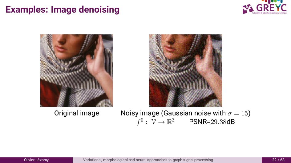
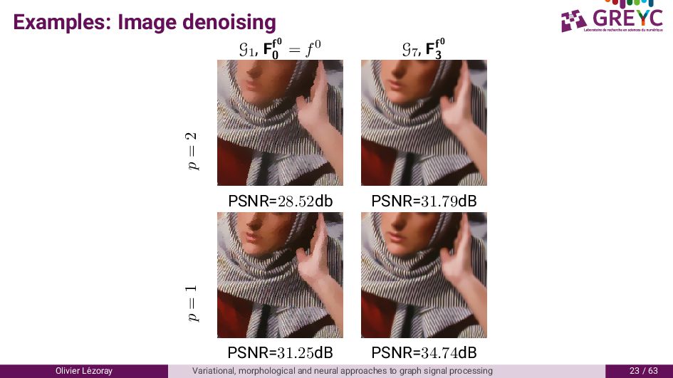
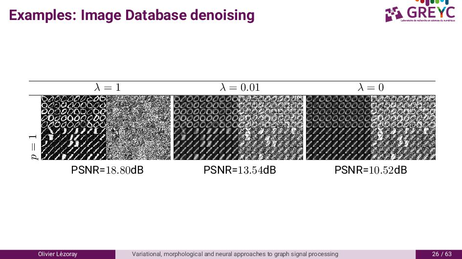
27. p-Laplacian nonlocal regularization on graphs Let f0 : V → R be the noisy version of a clean graph signal g : V → R defined on the vertices of a weighted graph G = (V, E, w). To recover g, seek for a function f : V → R regular enough on G, and close enough to f0, with the following variational problem: g ≈ min f:V→R Ew,p(f, f0, λ) = Rw,p(f) + λ 2 f − f0 2 2 , (8) where the regularization functional Rw,p is defined by the L2 norm of the gradient and is the discrete p-Dirichlet form of the function f ∈ H(V): Rw,p(f) = 1 p vi∈V (∇wf)(vi) p 2 = 1 p f, ∆i w,p f H(V) = 1 p vi∈V   vj∼vi wij(f(vj) − f(vi))2   p 2 . ( ) Olivier L´ ezoray Variational, morphological and neural approaches to graph signal processing / 6
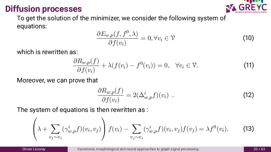
28. Diffusion processes To get the solution of the minimizer, we consider the following system of equations: ∂Ew,p(f, f0, λ) ∂f(vi) = 0, ∀vi ∈ V ( ) which is rewritten as: ∂Rw,p(f) ∂f(vi) + λ(f(vi) − f0(vi)) = 0, ∀vi ∈ V. ( ) Moreover, we can prove that ∂Rw,p(f) ∂f(vi) = 2(∆i w,p f)(vi) . ( ) The system of equations is then rewritten as :  λ + vj∼vi (γi w,p f)(vi, vj)   f(vi) − vj∼vi (γi w,p f)(vi, vj)f(vj) = λf0(vi). ( ) Olivier L´ ezoray Variational, morphological and neural approaches to graph signal processing / 6
29. Diffusion processes We can use the linearized Gauss-Jacobi iterative method to solve the previous systems. Let n be an iteration step, and let f(n) be the solution at the step n. Then, the method is given by the following algorithm:        f(0) = f0 f(n+1)(vi) = λf0(vi) + vj∼vi (γ∗ w,p f(n))(vi, vj)f(n)(vj) λ + vj∼vi (γ∗ w,p f(n))(vi, vj) , ∀vi ∈ V. ( ) with (γi w,p f)(vi, vj) = wij (∇wf)(vj) p−2 2 + (∇wf)(vi) p−2 2 , ( ) It describes a family of discrete diffusion processes, which is parameterized by the structure of the graph (topology and weight function), the parameter p, and the parameter λ. Olivier L´ ezoray Variational, morphological and neural approaches to graph signal processing / 6
30. Examples: Image denoising Original image Noisy image (Gaussian noise with σ = 15) f0 : V → R3 PSNR=29.38dB Olivier L´ ezoray Variational, morphological and neural approaches to graph signal processing / 6
31. Examples: Image denoising G1 , Ff0 0 = f0 G7 , Ff0 3 p = 2 PSNR=28.52db PSNR=31.79dB p = 1 PSNR=31.25dB PSNR=34.74dB Olivier L´ ezoray Variational, morphological and neural approaches to graph signal processing / 6
32. Examples: Mesh simplification Original Mesh p = 2 p = 1 f0 : V → R3 Olivier L´ ezoray Variational, morphological and neural approaches to graph signal processing / 6
33. Examples: Image Database denoising Initial data Noisy data -NNG f0 : V → R16×16 Olivier L´ ezoray Variational, morphological and neural approaches to graph signal processing / 6
34. Examples: Image Database denoising λ = 1 λ = 0.01 λ = 0 p = 1 PSNR=18.80dB PSNR=13.54dB PSNR=10.52dB Olivier L´ ezoray Variational, morphological and neural approaches to graph signal processing 6 / 6
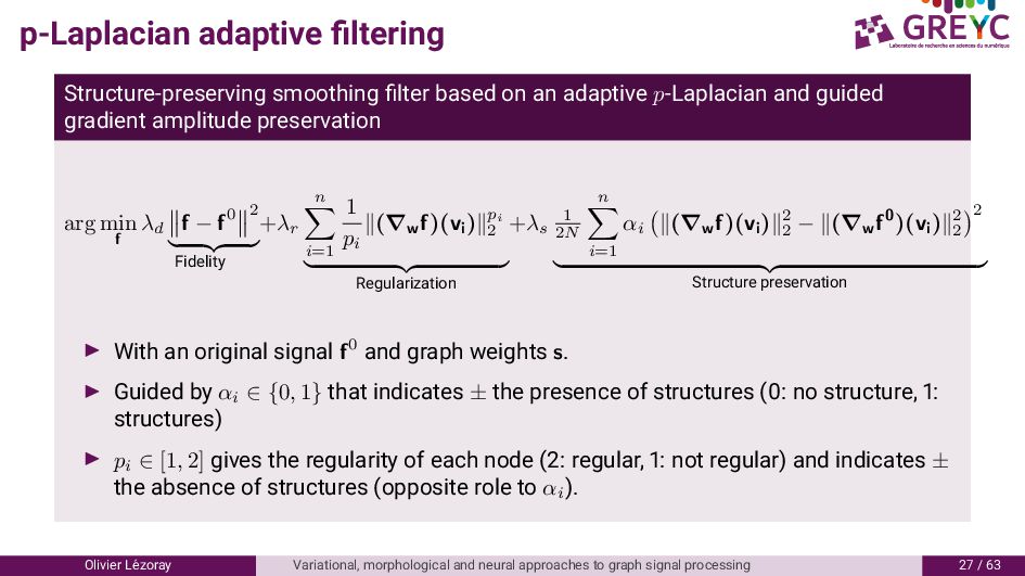
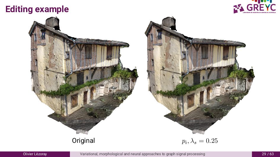
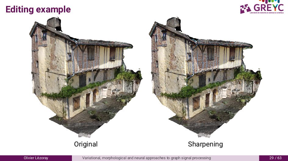
35. p-Laplacian adaptive filtering Structure-preserving smoothing filter based on an adaptive p-Laplacian and guided gradient amplitude preservation arg min f λd f − f0 2 Fidelity +λr n i=1 1 pi (∇w f)(vi ) pi 2 Regularization +λs 1 2N n i=1 αi (∇w f)(vi ) 2 2 − (∇w f0)(vi ) 2 2 2 Structure preservation With an original signal f0 and graph weights s. Guided by αi ∈ {0, 1} that indicates ± the presence of structures ( : no structure, : structures) pi ∈ [1, 2] gives the regularity of each node ( : regular, : not regular) and indicates ± the absence of structures (opposite role to αi ). Olivier L´ ezoray Variational, morphological and neural approaches to graph signal processing / 6
36. The regularity and structure indicators pi and αi are defined from a structure indicator mi using the Earth Mover Distance between the histograms of ρ-hop vectors Ff0 ρ (vi) in a τ-hop: mi := 1 |Nτ (vi)| vj∈Nτ (vi) dEMD(H(Ff0 ρ (vi)), H(Ff0 ρ (vj))) ( 6) pi := 1 + 1 1 + m2 i ( ) αi := mi − minj mj δi(maxj mj − minj mj) , δi out-degree of i in S ( 8) « pi and αi are antagonists : one for smoothing the data, the other for preserving the main structures Olivier L´ ezoray Variational, morphological and neural approaches to graph signal processing 8 / 6
37. Editing example Original Guide Olivier L´ ezoray Variational, morphological and neural approaches to graph signal processing / 6
38. Editing example Original pi, λs = 0.25 Olivier L´ ezoray Variational, morphological and neural approaches to graph signal processing / 6
39. Editing example Original Sharpening Olivier L´ ezoray Variational, morphological and neural approaches to graph signal processing / 6
40. Editing example Original Olivier L´ ezoray Variational, morphological and neural approaches to graph signal processing / 6
41. Editing example Original pi, λs = 0.25 Olivier L´ ezoray Variational, morphological and neural approaches to graph signal processing / 6
42. Editing example Original Sharpening Olivier L´ ezoray Variational, morphological and neural approaches to graph signal processing / 6
43. . Introduction . Notations . p-Laplacian adaptive filtering . Active contours on graphs . Morphological decomposition of graphs signals 6. Morphological segmentation of graph signals . Hand gesture recognition Olivier L´ ezoray Variational, morphological and neural approaches to graph signal processing / 6
44. Graph Signal Active contours Considered model We consider geometric approaches with level sets. Geodesic Active Contours An energy is associated to a curve C(p): EGAC(C) = 1 0 g(I(C(p)))|C (p)|dp Active Contours without edges Considers two regions separated by a curve, and minimizes: EACW E(C, c1, c2) = µ·Length(C)+ν·Area(inside(C))+λ1 inside(C) |I(x)−c1|2dx+λ2 outside(C) |I(x)−c2|2dx Considered active contours: combines both E(C, c1, c2) = µ 1 0 g(C(p))|C (p)|dp + ν · inside(C) g(C(p))dA + λ1 d inside(C) I(x) − c1 2 2 dx + λ2 d outside(C) I(x) − c2 2 2 dx This can be solved using a gradient descent from the associated Euler-Lagrange equations with the level-set framework. Olivier L´ ezoray Variational, morphological and neural approaches to graph signal processing / 6
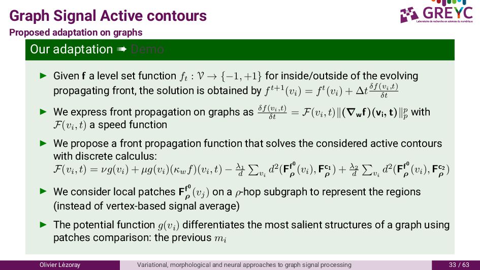
45. Graph Signal Active contours Proposed adaptation on graphs Our adaptation « Demo Given f a level set function ft : V → {−1, +1} for inside/outside of the evolving propagating front, the solution is obtained by ft+1(vi ) = ft(vi ) + ∆tδf(vi,t) δt We express front propagation on graphs as δf(vi,t) δt = F(vi , t) (∇w f)(vi , t) p p with F(vi , t) a speed function We propose a front propagation function that solves the considered active contours with discrete calculus: F(vi , t) = νg(vi ) + µg(vi )(κw f)(vi , t) − λ1 d vi d2(Ff0 ρ (vi ), Fc1 ρ ) + λ2 d vi d2(Ff0 ρ (vi ), Fc2 ρ ) We consider local patches Ff0 ρ (vj ) on a ρ-hop subgraph to represent the regions (instead of vertex-based signal average) The potential function g(vi ) differentiates the most salient structures of a graph using patches comparison: the previous mi Olivier L´ ezoray Variational, morphological and neural approaches to graph signal processing / 6
46. Results Grid Graph Signals (a) (b) (c) (d) (e) (f) Figure: From left to right: (a) Original image, (b) Checkerboard initialization, (c) GSAC; g(vi ) = 1, ρ = 0, (d) g(vi ), (e) GSAC; g(vi ), ρ = 0, (f) GSAC; g(vi ), ρ = 1. Olivier L´ ezoray Variational, morphological and neural approaches to graph signal processing / 6
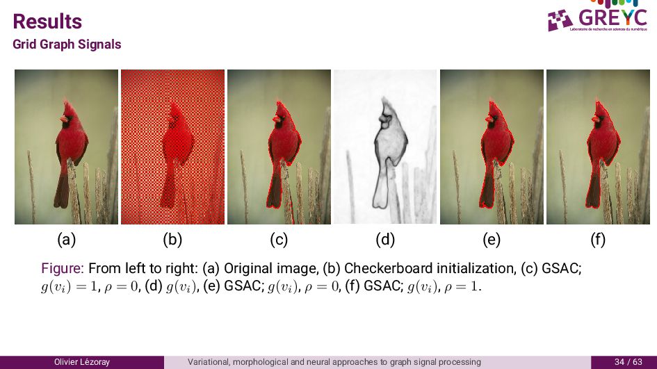
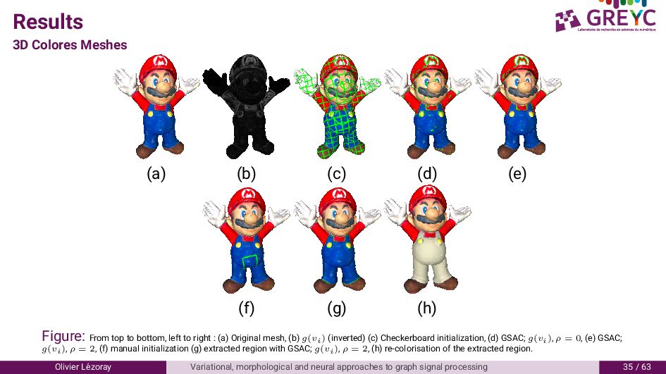
47. Results D Colores Meshes (a) (b) (c) (d) (e) (f) (g) (h) Figure: From top to bottom, left to right : (a) Original mesh, (b) g(vi) (inverted) (c) Checkerboard initialization, (d) GSAC; g(vi), ρ = 0, (e) GSAC; g(vi), ρ = 2, (f) manual initialization (g) extracted region with GSAC; g(vi), ρ = 2, (h) re-colorisation of the extracted region. Olivier L´ ezoray Variational, morphological and neural approaches to graph signal processing / 6
48. Results Image Dataset Graph Figure: Classification of a subset (digits and ) of the MNIST dataset. The colors around each image show the class it is affected to. The top row shows the initialization and bottom second row the final classification. 6 8 8.8 .8 . . . 6. . 6. Table: Classification scores for the 0 digit versus each other digit of the MNIST database. Olivier L´ ezoray Variational, morphological and neural approaches to graph signal processing 6 / 6
49. . Introduction . Notations . p-Laplacian adaptive filtering . Active contours on graphs . Morphological decomposition of graphs signals 6. Morphological segmentation of graph signals . Hand gesture recognition Olivier L´ ezoray Variational, morphological and neural approaches to graph signal processing / 6
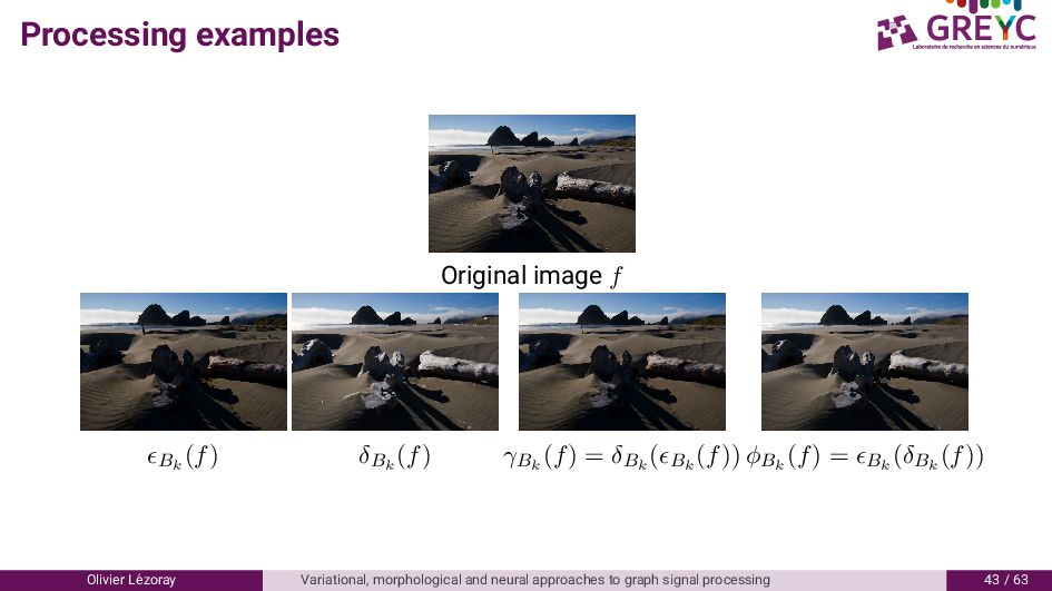
50. Introduction - Mathematical Morphology Fundamental operators in Mathematical Morphology (MM) are dilation and erosion. Dilation δ of a function f0 : Ω ⊂ R2 → R consists in replacing the function value by the maximum value within a structuring element B such that: δB f0(x, y) = max f0(x + x , y + y )|(x , y ) ∈ B Erosion is computed by: B f0(x, y) = min f0(x + x , y + y )|(x , y ) ∈ B Olivier L´ ezoray Variational, morphological and neural approaches to graph signal processing 8 / 6
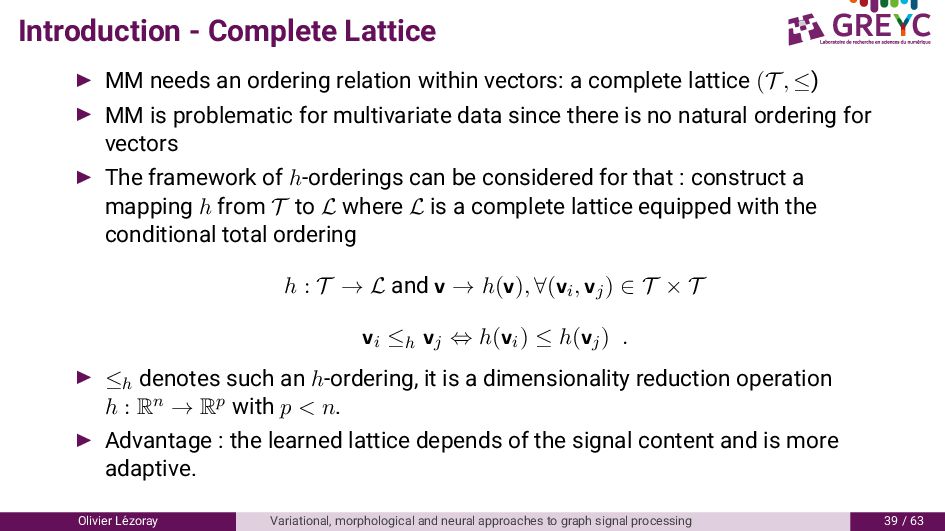
51. Introduction - Complete Lattice MM needs an ordering relation within vectors: a complete lattice (T , ≤) MM is problematic for multivariate data since there is no natural ordering for vectors The framework of h-orderings can be considered for that : construct a mapping h from T to L where L is a complete lattice equipped with the conditional total ordering h : T → L and v → h(v), ∀(vi, vj) ∈ T × T vi ≤h vj ⇔ h(vi) ≤ h(vj) . ≤h denotes such an h-ordering, it is a dimensionality reduction operation h : Rn → Rp with p < n. Advantage : the learned lattice depends of the signal content and is more adaptive. Olivier L´ ezoray Variational, morphological and neural approaches to graph signal processing / 6
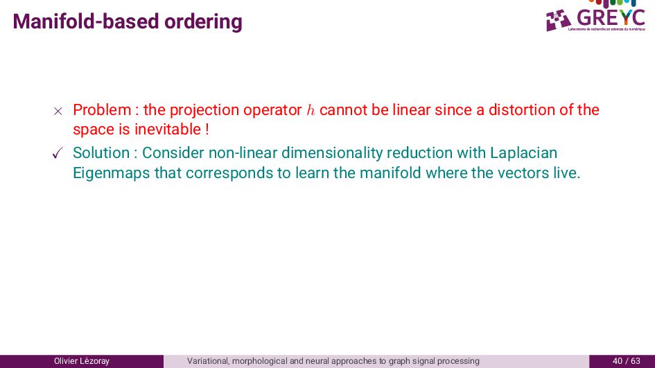
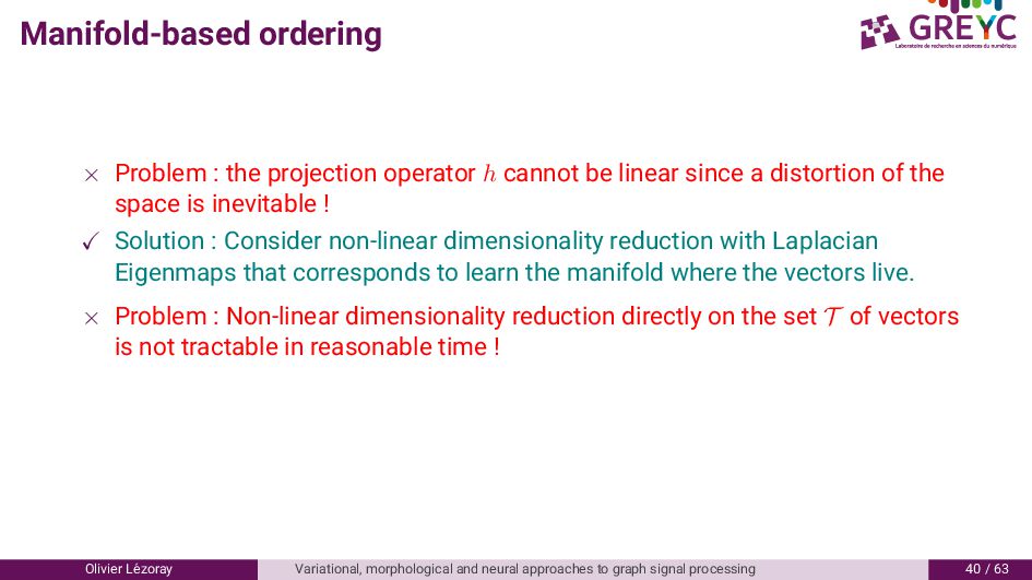
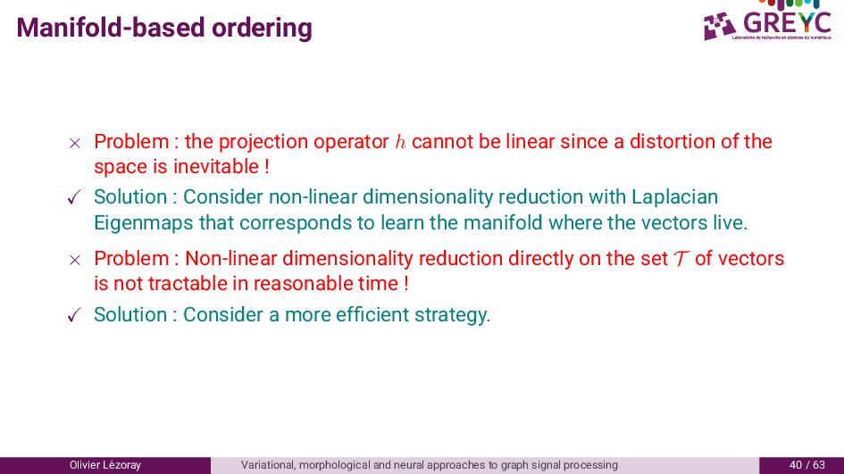
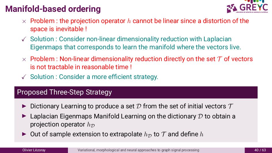
52. Manifold-based ordering × Problem : the projection operator h cannot be linear since a distortion of the space is inevitable ! Olivier L´ ezoray Variational, morphological and neural approaches to graph signal processing / 6
53. Manifold-based ordering × Problem : the projection operator h cannot be linear since a distortion of the space is inevitable ! Solution : Consider non-linear dimensionality reduction with Laplacian Eigenmaps that corresponds to learn the manifold where the vectors live. Olivier L´ ezoray Variational, morphological and neural approaches to graph signal processing / 6
54. Manifold-based ordering × Problem : the projection operator h cannot be linear since a distortion of the space is inevitable ! Solution : Consider non-linear dimensionality reduction with Laplacian Eigenmaps that corresponds to learn the manifold where the vectors live. × Problem : Non-linear dimensionality reduction directly on the set T of vectors is not tractable in reasonable time ! Olivier L´ ezoray Variational, morphological and neural approaches to graph signal processing / 6
55. Manifold-based ordering × Problem : the projection operator h cannot be linear since a distortion of the space is inevitable ! Solution : Consider non-linear dimensionality reduction with Laplacian Eigenmaps that corresponds to learn the manifold where the vectors live. × Problem : Non-linear dimensionality reduction directly on the set T of vectors is not tractable in reasonable time ! Solution : Consider a more efficient strategy. Olivier L´ ezoray Variational, morphological and neural approaches to graph signal processing / 6
56. Manifold-based ordering × Problem : the projection operator h cannot be linear since a distortion of the space is inevitable ! Solution : Consider non-linear dimensionality reduction with Laplacian Eigenmaps that corresponds to learn the manifold where the vectors live. × Problem : Non-linear dimensionality reduction directly on the set T of vectors is not tractable in reasonable time ! Solution : Consider a more efficient strategy. Proposed Three-Step Strategy Dictionary Learning to produce a set D from the set of initial vectors T Laplacian Eigenmaps Manifold Learning on the dictionary D to obtain a projection operator hD Out of sample extension to extrapolate hD to T and define h Olivier L´ ezoray Variational, morphological and neural approaches to graph signal processing / 6
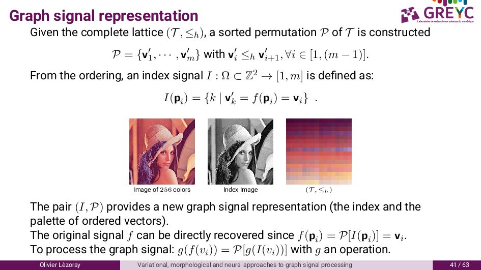
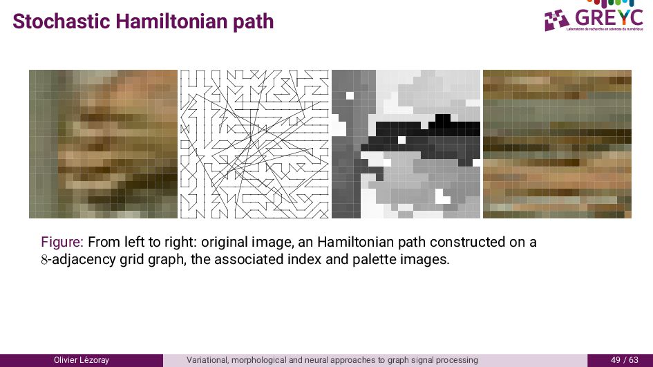
57. Graph signal representation Given the complete lattice (T , ≤h), a sorted permutation P of T is constructed P = {v1 , · · · , vm } with vi ≤h vi+1 , ∀i ∈ [1, (m − 1)]. From the ordering, an index signal I : Ω ⊂ Z2 → [1, m] is defined as: I(pi ) = {k | vk = f(pi ) = vi} . Image of 256 colors Index Image (T , ≤h) The pair (I, P) provides a new graph signal representation (the index and the palette of ordered vectors). The original signal f can be directly recovered since f(pi ) = P[I(pi )] = vi . To process the graph signal: g(f(vi)) = P[g(I(vi))] with g an operation. Olivier L´ ezoray Variational, morphological and neural approaches to graph signal processing / 6
58. Examples of obtained representations Olivier L´ ezoray Variational, morphological and neural approaches to graph signal processing / 6
59. Examples of obtained representations Olivier L´ ezoray Variational, morphological and neural approaches to graph signal processing / 6
60. Processing examples Original image f Bk (f) δBk (f) γBk (f) = δBk ( Bk (f)) φBk (f) = Bk (δBk (f)) Olivier L´ ezoray Variational, morphological and neural approaches to graph signal processing / 6
61. Processing examples Original colored mesh f Bk (f) δBk (f) γBk (f) = δBk ( Bk (f)) φBk (f) = Bk (δBk (f)) Olivier L´ ezoray Variational, morphological and neural approaches to graph signal processing / 6
62. Image and Mesh abstraction Performed with an OCCO filter. Olivier L´ ezoray Variational, morphological and neural approaches to graph signal processing / 6
63. Image and Mesh abstraction Performed with an OCCO filter. Olivier L´ ezoray Variational, morphological and neural approaches to graph signal processing / 6
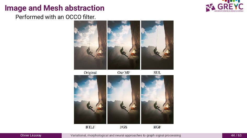
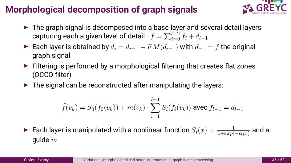
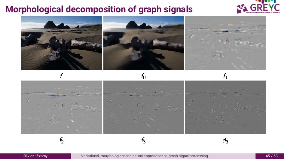
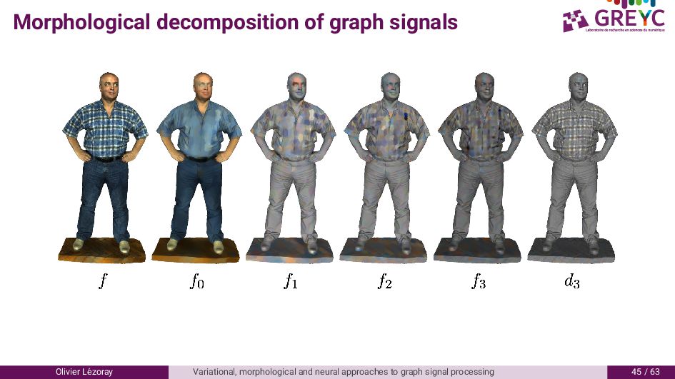
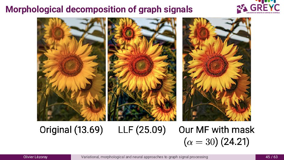
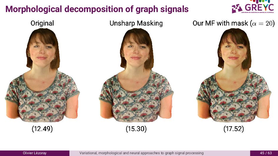
64. Morphological decomposition of graph signals The graph signal is decomposed into a base layer and several detail layers capturing each a given level of detail : f = l−2 i=0 fi + dl−1 Each layer is obtained by di = di−1 − FM(di−1) with d−1 = f the original graph signal Filtering is performed by a morphological filtering that creates flat zones (OCCO filter) The signal can be reconstructed after manipulating the layers: ˆ f(vk) = S0(f0(vk)) + m(vk) · l−1 i=1 Si(fi(vk)) avec fl−1 = dl−1 Each layer is manipulated with a nonlinear function Si(x) = 1 1+exp(−αix) and a guide m Olivier L´ ezoray Variational, morphological and neural approaches to graph signal processing / 6
65. Morphological decomposition of graph signals Olivier L´ ezoray Variational, morphological and neural approaches to graph signal processing / 6
66. Morphological decomposition of graph signals Olivier L´ ezoray Variational, morphological and neural approaches to graph signal processing / 6
67. Morphological decomposition of graph signals Olivier L´ ezoray Variational, morphological and neural approaches to graph signal processing / 6
68. Morphological decomposition of graph signals Olivier L´ ezoray Variational, morphological and neural approaches to graph signal processing / 6
69. . Introduction . Notations . p-Laplacian adaptive filtering . Active contours on graphs . Morphological decomposition of graphs signals 6. Morphological segmentation of graph signals . Hand gesture recognition Olivier L´ ezoray Variational, morphological and neural approaches to graph signal processing 6 / 6
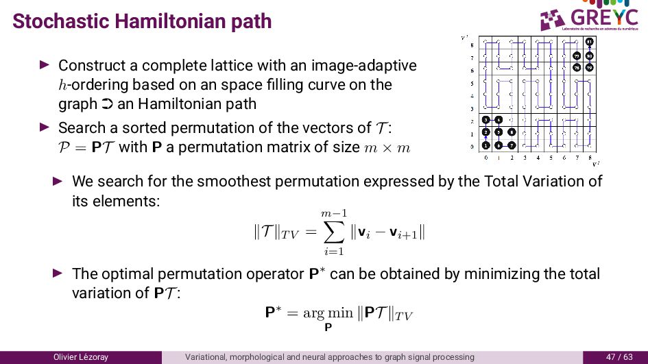
70. Stochastic Hamiltonian path Construct a complete lattice with an image-adaptive h-ordering based on an space filling curve on the graph · an Hamiltonian path Search a sorted permutation of the vectors of T : P = PT with P a permutation matrix of size m × m We search for the smoothest permutation expressed by the Total Variation of its elements: T TV = m−1 i=1 vi − vi+1 The optimal permutation operator P∗ can be obtained by minimizing the total variation of PT : P∗ = arg min P PT TV Olivier L´ ezoray Variational, morphological and neural approaches to graph signal processing / 6
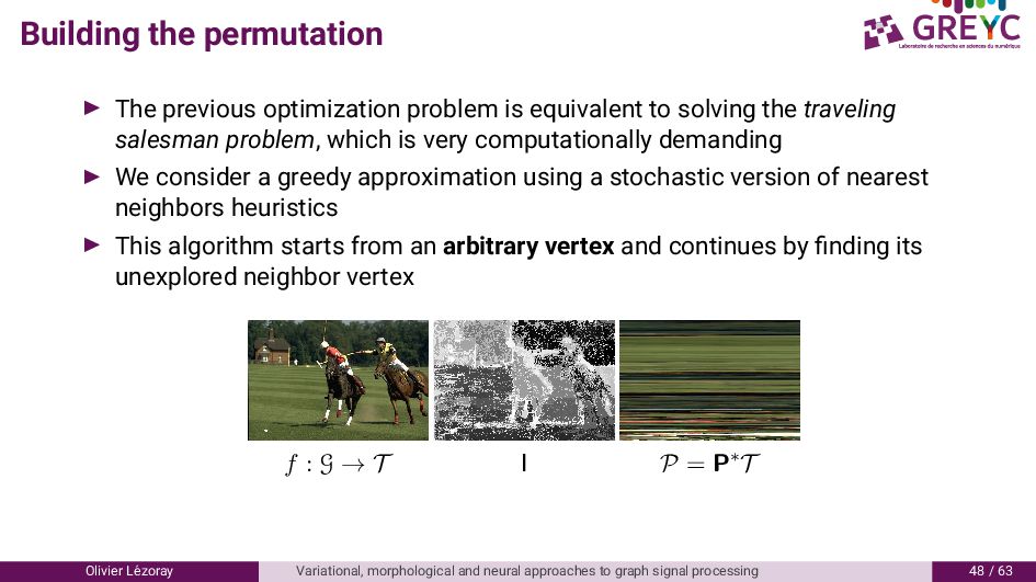
71. Building the permutation The previous optimization problem is equivalent to solving the traveling salesman problem, which is very computationally demanding We consider a greedy approximation using a stochastic version of nearest neighbors heuristics This algorithm starts from an arbitrary vertex and continues by finding its unexplored neighbor vertex f : G → T I P = P∗T Olivier L´ ezoray Variational, morphological and neural approaches to graph signal processing 8 / 6
72. Stochastic Hamiltonian path 0 1 20 21 2 3 22 23 4 5 24 25 6 26 27 7 8 28 9 10 30 29 11 367 12 13 31 32 14 15 136 55 16 17 37 18 19 39 40 41 42 43 375 45 47 50 52 33 34 54 53 35 36 38 59 60 44 63 64 46 66 67 48 49 69 70 51 71 74 75 56 57 76 58 77 79 80 61 81 82 62 120 259 83 65 85 86 68 87 88 89 91 72 73 93 94 95 78 100 101 103 84 104 165 99 108 90 111 92 96 97 116 117 98 224 102 121 123 105 124 106 125 127 107 110 109 189 112 113 114 115 118 119 139 161 122 142 143 144 126 145 128 129 130 131 132 133 152 134 153 154 135 155 156 285 137 138 249 140 160 366 141 162 163 164 146 166 167 147 148 149 150 170 151 171 284 157 158 159 179 182 183 184 168 169 188 172 173 174 175 176 177 178 180 181 200 241 201 203 185 186 204 207 187 206 324 190 209 210 191 192 213 193 194 214 195 196 197 198 199 218 202 221 222 205 208 211 212 232 215 216 237 217 266 219 239 220 240 223 242 245 225 226 394 246 227 228 248 229 230 231 250 233 234 235 236 257 238 258 261 260 262 243 244 263 264 247 354 270 251 271 272 252 253 273 254 274 275 255 256 276 334 280 282 281 283 265 286 267 287 288 268 269 293 294 277 278 279 299 300 301 302 303 304 289 290 311 291 292 310 295 296 315 297 298 316 321 323 305 306 326 307 308 309 312 331 333 313 314 332 317 318 319 339 320 340 341 322 342 343 325 344 346 327 347 328 329 348 330 352 353 355 335 336 356 357 337 338 360 361 363 345 364 368 349 350 371 351 372 376 358 359 377 379 380 362 382 383 384 365 385 386 387 389 369 370 388 391 373 374 395 396 378 397 399 398 381 390 392 393 Figure: From left to right: original image, an Hamiltonian path constructed on a 8-adjacency grid graph, the associated index and palette images. Olivier L´ ezoray Variational, morphological and neural approaches to graph signal processing / 6
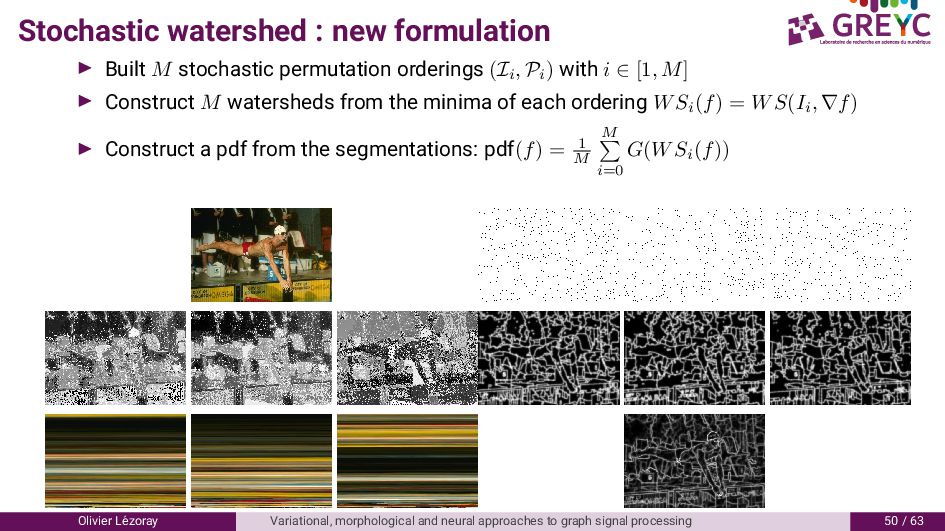
73. Stochastic watershed : new formulation Built M stochastic permutation orderings (Ii , Pi ) with i ∈ [1, M] Construct M watersheds from the minima of each ordering WSi (f) = WS(Ii , ∇f) Construct a pdf from the segmentations: pdf(f) = 1 M M i=0 G(WSi (f)) Olivier L´ ezoray Variational, morphological and neural approaches to graph signal processing / 6
74. Examples Original image Color combined gradient gc Patch combined gradient gp Seeds Watershed with gc Watershed with gradient gp Figure: Segmentation examples with our stochastic permutation watershed. Olivier L´ ezoray Variational, morphological and neural approaches to graph signal processing / 6
75. An application Bayeux tapestry Historians need to interactively delineate some characters in the tapestry images A precise segmentation is required by using simple object/background seed labeling by point click to ease the end-users use The characters are visually easy to identify but the reduced number of colors, the fine embroidery as well as the texture differences in the linen fabric can make the segmentation hard. The permutation based stochastic watershed is performed with 7 × 7 patches Olivier L´ ezoray Variational, morphological and neural approaches to graph signal processing / 6
76. . Introduction . Notations . p-Laplacian adaptive filtering . Active contours on graphs . Morphological decomposition of graphs signals 6. Morphological segmentation of graph signals . Hand gesture recognition Olivier L´ ezoray Variational, morphological and neural approaches to graph signal processing / 6
77. Hand gesture recognition Olivier L´ ezoray Variational, morphological and neural approaches to graph signal processing / 6
78. Hand gesture recognition Olivier L´ ezoray Variational, morphological and neural approaches to graph signal processing / 6
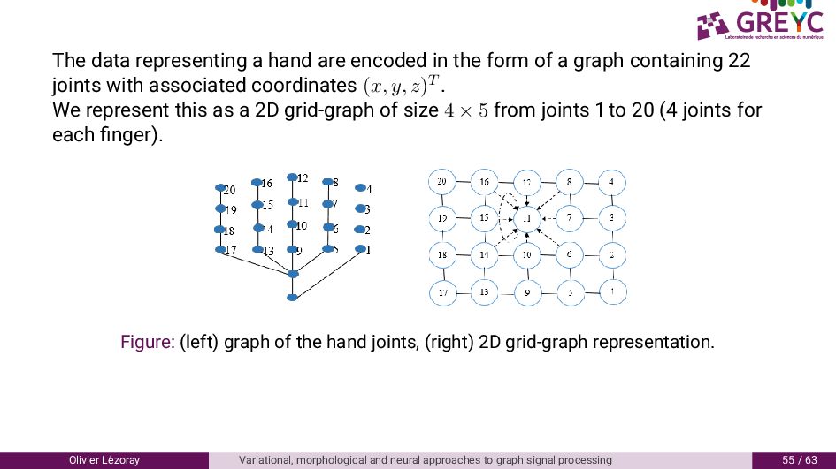
79. The data representing a hand are encoded in the form of a graph containing joints with associated coordinates (x, y, z)T . We represent this as a D grid-graph of size 4 × 5 from joints to ( joints for each finger). Figure: (left) graph of the hand joints, (right) D grid-graph representation. Olivier L´ ezoray Variational, morphological and neural approaches to graph signal processing / 6
80. We have video sequences of gestures and therefore each frame corresponds to a grid. They are processed using a deep network Figure: DeepSPDNet. Olivier L´ ezoray Variational, morphological and neural approaches to graph signal processing 6 / 6
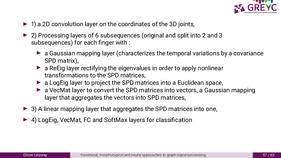
81. ) a D convolution layer on the coordinates of the D joints, ) Processing layers of 6 subsequences (original and split into and subsequences) for each finger with : a Gaussian mapping layer (characterizes the temporal variations by a covariance SPD matrix), a ReEig layer rectifying the eigenvalues in order to apply nonlinear transformations to the SPD matrices, a LogEig layer to project the SPD matrices into a Euclidean space, a VecMat layer to convert the SPD matrices into vectors, a Gaussian mapping layer that aggregates the vectors into SPD matrices, ) A linear mapping layer that aggregates the SPD matrices into one, ) LogEig, VecMat, FC and SoftMax layers for classification Olivier L´ ezoray Variational, morphological and neural approaches to graph signal processing / 6
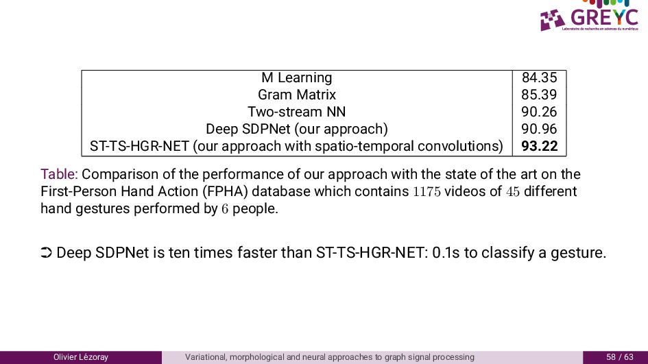
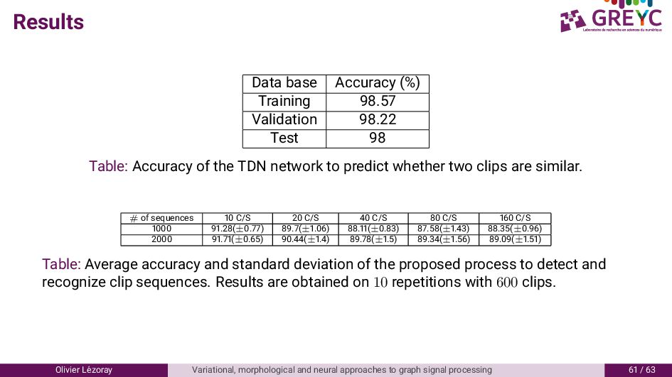
82. M Learning 8 . Gram Matrix 8 . Two-stream NN . 6 Deep SDPNet (our approach) . 6 ST-TS-HGR-NET (our approach with spatio-temporal convolutions) . Table: Comparison of the performance of our approach with the state of the art on the First-Person Hand Action (FPHA) database which contains 1175 videos of 45 different hand gestures performed by 6 people. · Deep SDPNet is ten times faster than ST-TS-HGR-NET: . s to classify a gesture. Olivier L´ ezoray Variational, morphological and neural approaches to graph signal processing 8 / 6
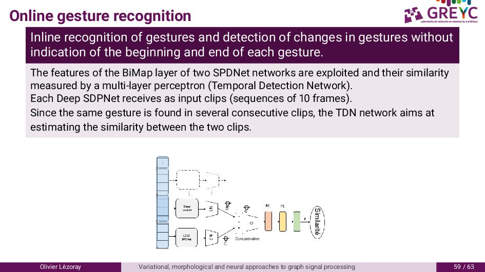
83. Online gesture recognition Inline recognition of gestures and detection of changes in gestures without indication of the beginning and end of each gesture. The features of the BiMap layer of two SPDNet networks are exploited and their similarity measured by a multi-layer perceptron (Temporal Detection Network). Each Deep SDPNet receives as input clips (sequences of frames). Since the same gesture is found in several consecutive clips, the TDN network aims at estimating the similarity between the two clips. Olivier L´ ezoray Variational, morphological and neural approaches to graph signal processing / 6
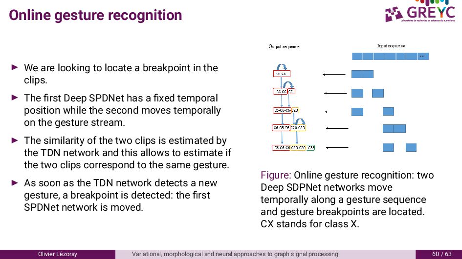
84. Online gesture recognition We are looking to locate a breakpoint in the clips. The first Deep SPDNet has a fixed temporal position while the second moves temporally on the gesture stream. The similarity of the two clips is estimated by the TDN network and this allows to estimate if the two clips correspond to the same gesture. As soon as the TDN network detects a new gesture, a breakpoint is detected: the first SPDNet network is moved. Figure: Online gesture recognition: two Deep SDPNet networks move temporally along a gesture sequence and gesture breakpoints are located. CX stands for class X. Olivier L´ ezoray Variational, morphological and neural approaches to graph signal processing 6 / 6
85. Results Data base Accuracy (%) Training 8. Validation 8. Test 8 Table: Accuracy of the TDN network to predict whether two clips are similar. # of sequences C/S C/S C/S 8 C/S 6 C/S . 8(± . ) 8 . (± . 6) 88. (± .8 ) 8 . 8(± . ) 88. (± . 6) . (± .6 ) . (± . ) 8 . 8(± . ) 8 . (± . 6) 8 . (± . ) Table: Average accuracy and standard deviation of the proposed process to detect and recognize clip sequences. Results are obtained on 10 repetitions with 600 clips. Olivier L´ ezoray Variational, morphological and neural approaches to graph signal processing 6 / 6
86. Application in Virtual Reality Ancient Automata : The maidservant of Philo of Byzantium ( BC) Olivier L´ ezoray Variational, morphological and neural approaches to graph signal processing 6 / 6
87. Application in Virtual Reality Ancient Automata : The maidservant of Philo of Byzantium ( BC) Olivier L´ ezoray Variational, morphological and neural approaches to graph signal processing 6 / 6
88. Application in Virtual Reality Ancient Automata : The maidservant of Philo of Byzantium ( BC) Demo Olivier L´ ezoray Variational, morphological and neural approaches to graph signal processing 6 / 6
89. The end [thank you] Any Questions ? olivier.lezoray@unicaen.fr https://lezoray.users.greyc.fr Olivier L´ ezoray Variational, morphological and neural approaches to graph signal processing 6 / 6