ICube Strasbourg Seminar 2017

Transcript

1. Saliency-based 3D data processing Olivier L´ ezoray Normandie Univ, UNICAEN, ENSICAEN, CNRS, GREYC, 14000 Caen, France olivier.lezoray@unicaen.fr https://lezoray.users.greyc.fr
2. 1 Introduction 2 3D Data Saliency 3 3D Point Cloud Colorization 4 3D Colored Mesh Enhancement 5 Conclusion 2 / 64
3. 1 Introduction 2 3D Data Saliency 3 3D Point Cloud Colorization 4 3D Colored Mesh Enhancement 5 Conclusion 3 / 64
4. Introduction Recent technological advances have lead to the generation of huge amounts of 3D data Even with cheap hardware and software, one can easily generate 3D data 4 / 64
5. Introduction Recent technological advances have lead to the generation of huge amounts of 3D data Even with cheap hardware and software, one can easily generate 3D data 3D data acquisition with common smartphone (Technology: Photogrammetry) 4 / 64
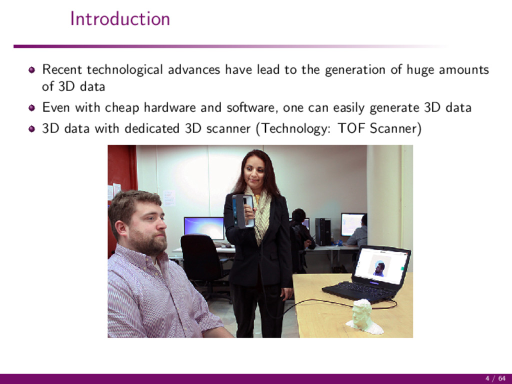
6. Introduction Recent technological advances have lead to the generation of huge amounts of 3D data Even with cheap hardware and software, one can easily generate 3D data 3D data with dedicated 3D scanner (Technology: TOF Scanner) 4 / 64
7. Introduction Recent technological advances have lead to the generation of huge amounts of 3D data Even with cheap hardware and software, one can easily generate 3D data 3D data with dedicated 3D scanner (Technology: Laser Scanner) 4 / 64
8. New applications Fields With this proliferation of such 3D Data, new application fields have appeared 5 / 64
9. New applications Fields With this proliferation of such 3D Data, new application fields have appeared 3D Digital Forensics : 3D scans of a crime scenes for police investigations 5 / 64
10. New applications Fields With this proliferation of such 3D Data, new application fields have appeared 3D Culturage Heritage : 3D scans of cultural heritage sites for memory preservation 5 / 64
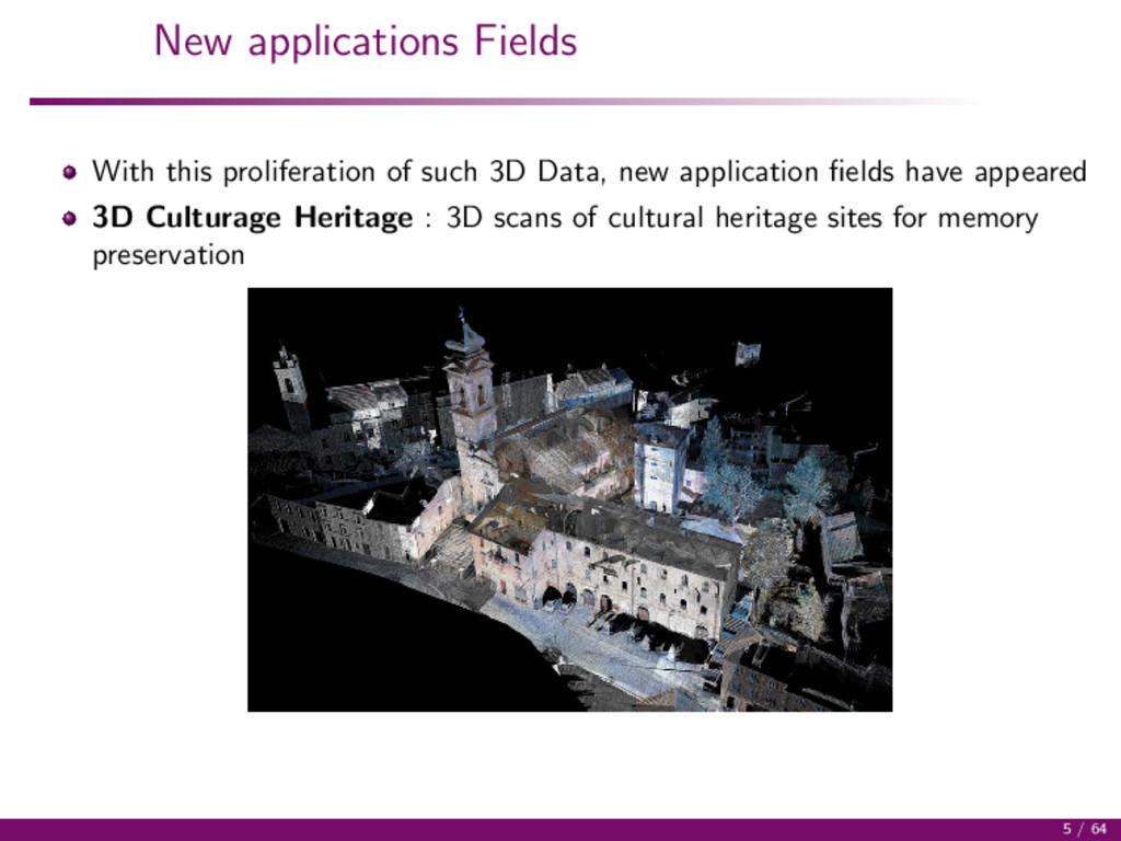
11. New applications Fields With this proliferation of such 3D Data, new application fields have appeared 3D Body Scanning : 3D body scanning for movie and game production, avatar creation, medical industry, fashion industry, 5 / 64
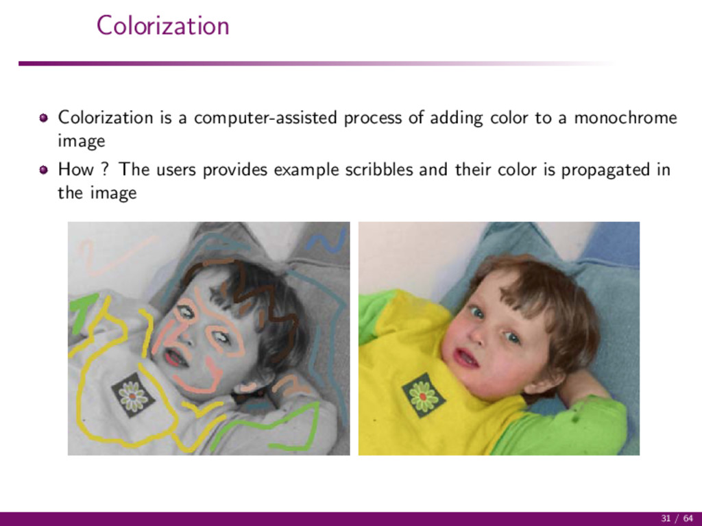
12. New challenging problems Many different 3D data formats : point clouds or meshes with attached coordinates, color per vertex or texture per face In this talk: 3D point clouds or meshes with coordinates and color information per vertex Most classical inverse problems in computer vision find their analogue with 3D (colored) point clouds (denoising, inpainting, segmentation, matching, ...) In this talk: viewpoint selection, colorization, and sharpening with the use of 3D saliency information 6 / 64
13. 1 Introduction 2 3D Data Saliency 3 3D Point Cloud Colorization 4 3D Colored Mesh Enhancement 5 Conclusion 7 / 64
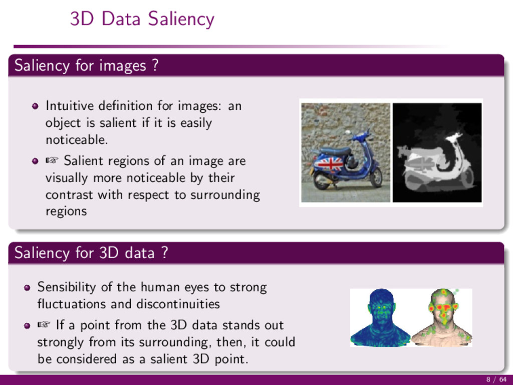
14. 3D Data Saliency Saliency for images ? Intuitive definition for images: an object is salient if it is easily noticeable. Salient regions of an image are visually more noticeable by their contrast with respect to surrounding regions Saliency for 3D data ? Sensibility of the human eyes to strong fluctuations and discontinuities If a point from the 3D data stands out strongly from its surrounding, then, it could be considered as a salient 3D point. 8 / 64
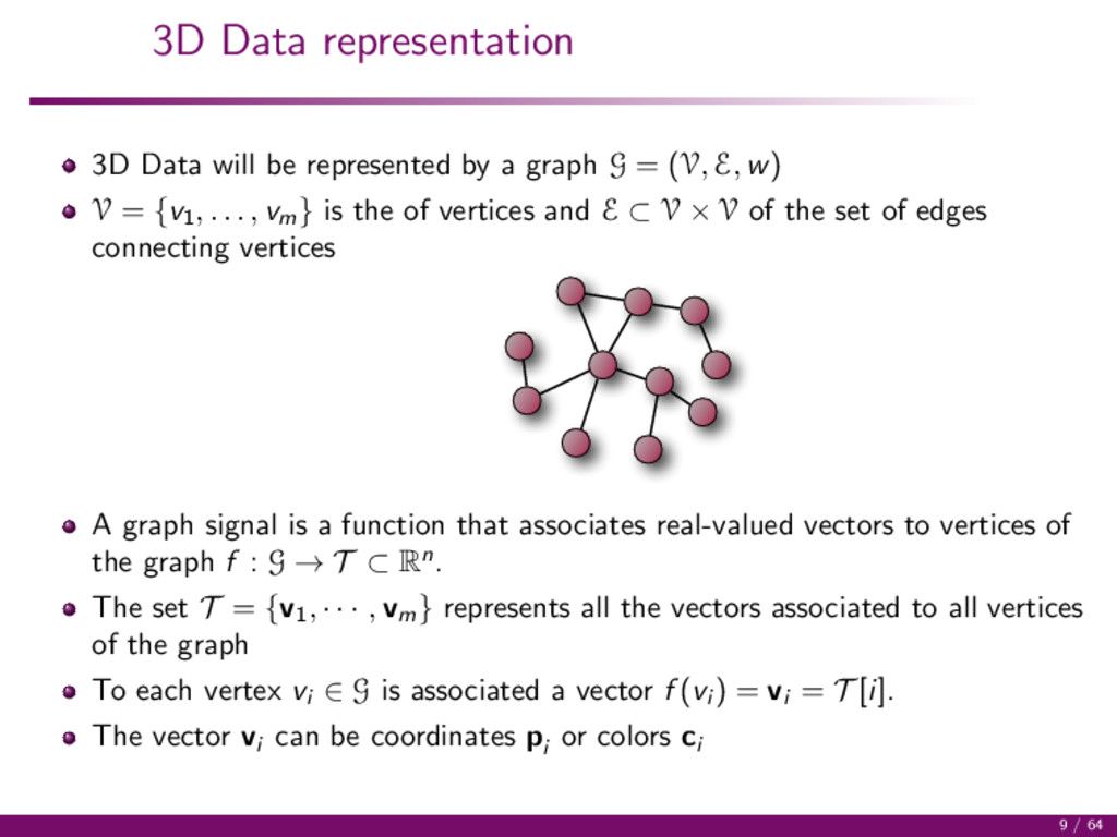
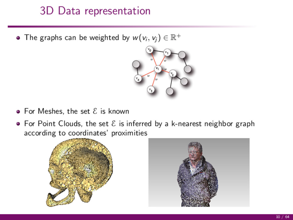
15. 3D Data representation 3D Data will be represented by a graph G = (V, E, w) V = {v1, . . . , vm} is the of vertices and E ⊂ V × V of the set of edges connecting vertices A graph signal is a function that associates real-valued vectors to vertices of the graph f : G → T ⊂ Rn. The set T = {v1, · · · , vm} represents all the vectors associated to all vertices of the graph To each vertex vi ∈ G is associated a vector f (vi ) = vi = T [i]. The vector vi can be coordinates pi or colors ci 9 / 64
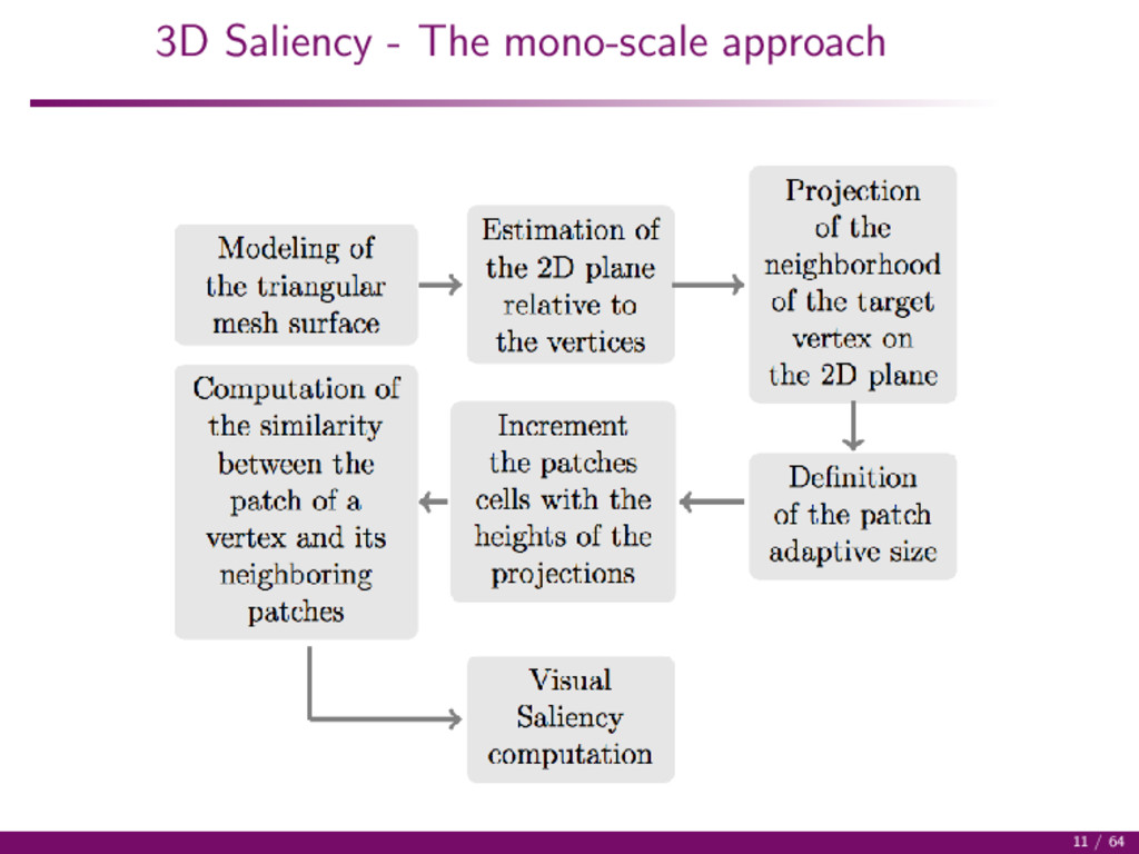
16. 3D Data representation The graphs can be weighted by w(vi , vj ) ∈ R+ For Meshes, the set E is known For Point Clouds, the set E is inferred by a k-nearest neighbor graph according to coordinates’ proximities 10 / 64
17. 3D Saliency - The mono-scale approach 11 / 64
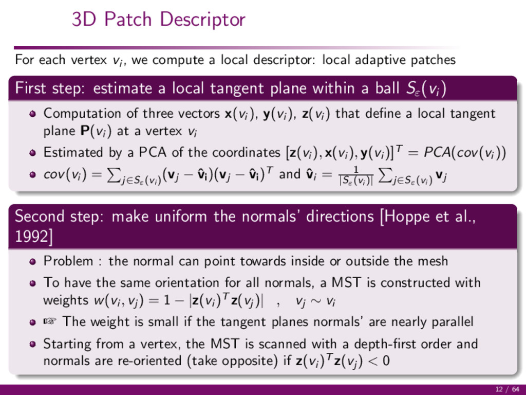
18. 3D Patch Descriptor For each vertex vi , we compute a local descriptor: local adaptive patches First step: estimate a local tangent plane within a ball Sε (vi ) Computation of three vectors x(vi ), y(vi ), z(vi ) that define a local tangent plane P(vi ) at a vertex vi Estimated by a PCA of the coordinates [z(vi ), x(vi ), y(vi )]T = PCA(cov(vi )) cov(vi ) = j∈Sε(vi ) (vj − ˆ vi )(vj − ˆ vi )T and ˆ vi = 1 |Sε(vi )| j∈Sε(vi ) vj Second step: make uniform the normals’ directions [Hoppe et al., 1992] Problem : the normal can point towards inside or outside the mesh To have the same orientation for all normals, a MST is constructed with weights w(vi , vj ) = 1 − |z(vi )T z(vj )| , vj ∼ vi The weight is small if the tangent planes normals’ are nearly parallel Starting from a vertex, the MST is scanned with a depth-first order and normals are re-oriented (take opposite) if z(vi )T z(vj ) < 0 12 / 64
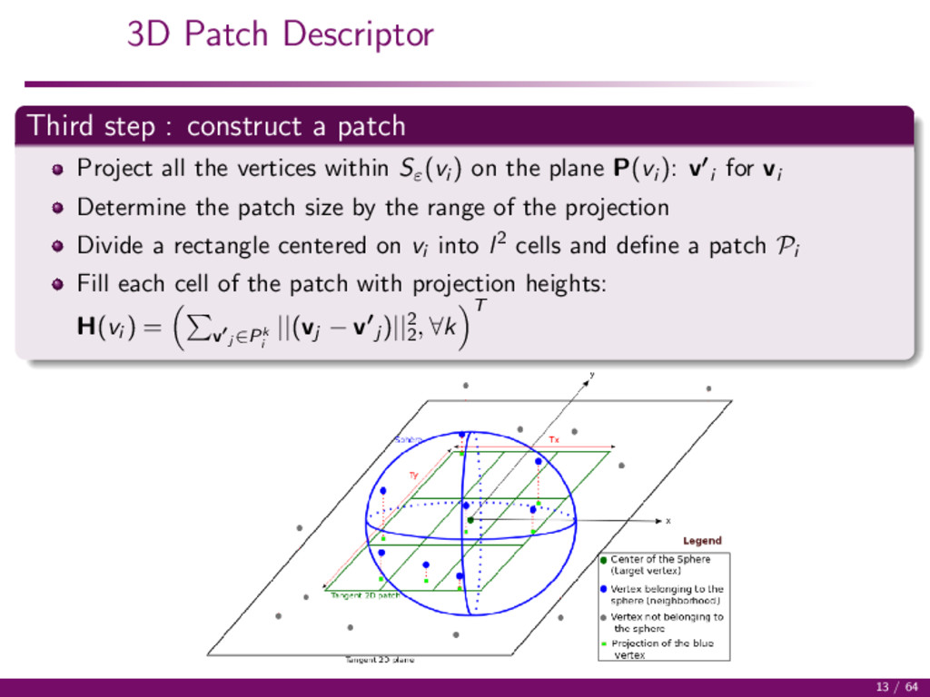
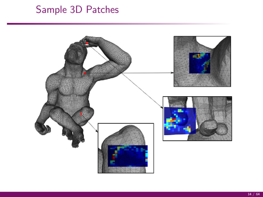
19. 3D Patch Descriptor Third step : construct a patch Project all the vertices within Sε (vi ) on the plane P(vi ): v i for vi Determine the patch size by the range of the projection Divide a rectangle centered on vi into l2 cells and define a patch Pi Fill each cell of the patch with projection heights: H(vi ) = v j ∈Pk i ||(vj − v j )||2 2 , ∀k T 13 / 64
20. Sample 3D Patches 14 / 64
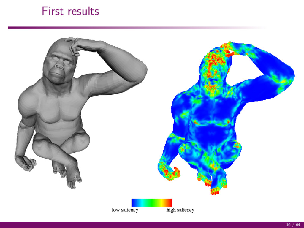
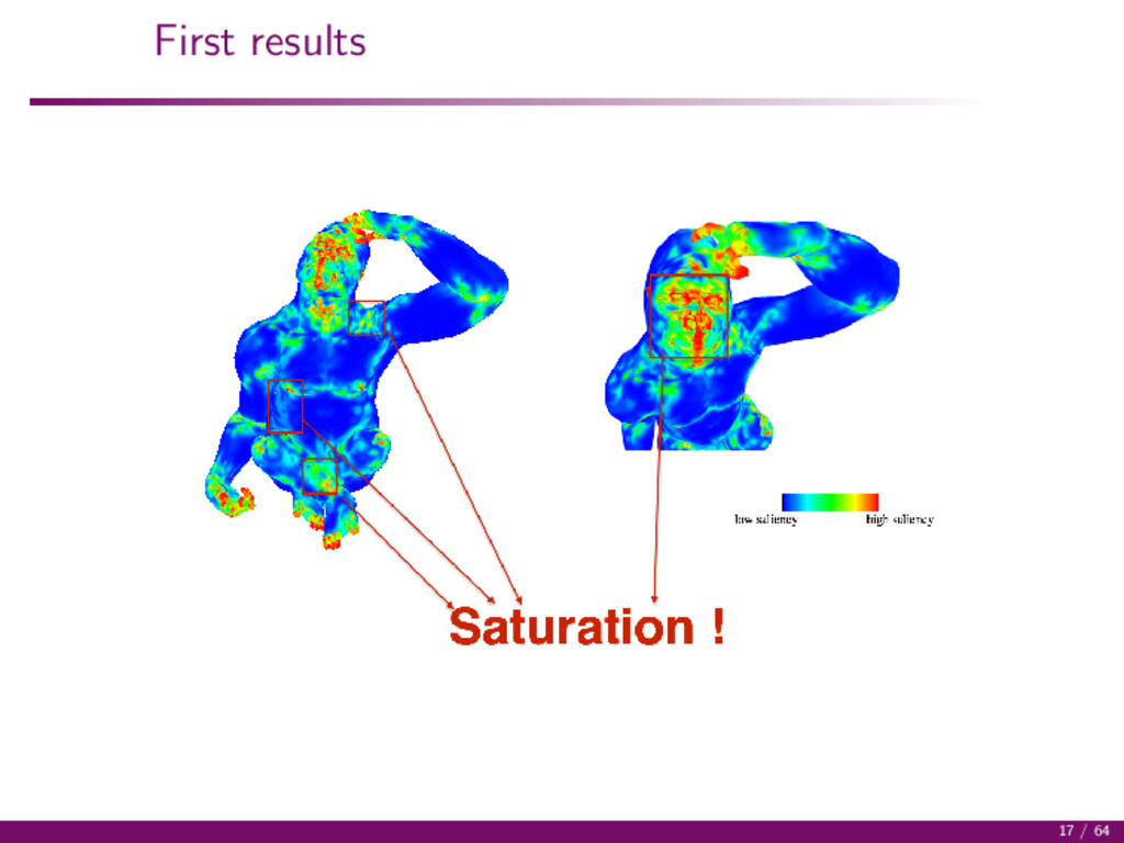
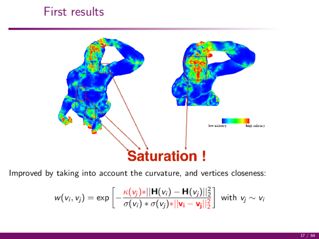
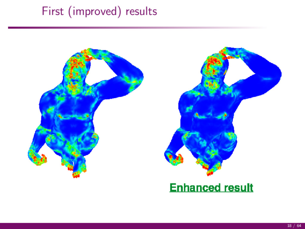
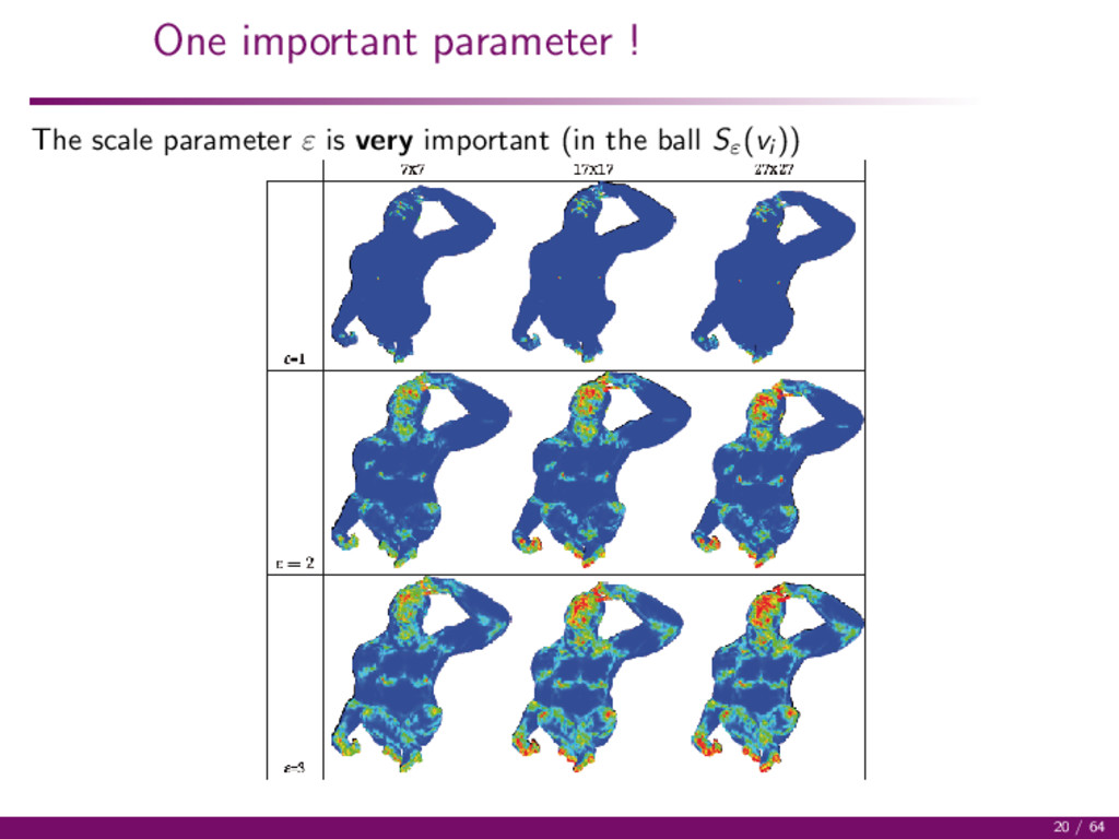
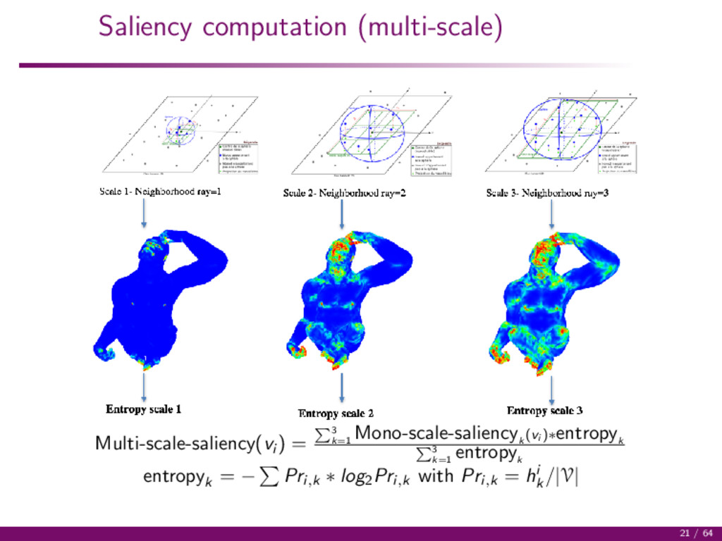
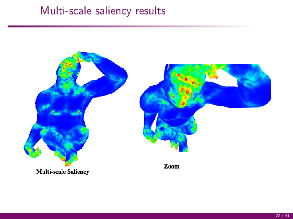
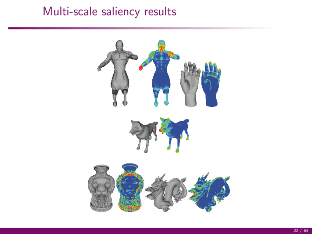
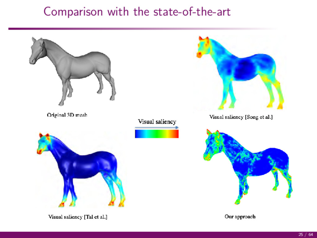
21. Saliency computation (single-scale) Compute weights on the graph G associated to the 3D data: w(vi , vj ) = exp − ||H(vi ) − H(vj )||2 2 σ(vi ) ∗ σ(vj ) with vj ∼ vi Automatic scale parameter: σ(vi ) = maxvk ∼vi (||vi − vk ||2 ) The single-scale saliency is defined as the average degree of a vertex vi : Mono-scale-saliency(vi ) = 1 |vj ∼ vi | vi ∼vj w(vi , vj ) Close to 0: salient Close to 1: not salient 15 / 64
22. First results 16 / 64
23. First results 17 / 64
24. First results Improved by taking into account the curvature, and vertices closeness: w(vi , vj ) = exp − κ(vj )∗||H(vi ) − H(vj )||2 2 σ(vi ) ∗ σ(vj )∗||vi − vj||2 2 with vj ∼ vi 17 / 64
25. First (improved) results 18 / 64
26. First (improved) results 19 / 64
27. One important parameter ! The scale parameter ε is very important (in the ball Sε (vi )) 20 / 64
28. Saliency computation (multi-scale) Multi-scale-saliency(vi ) = 3 k=1 Mono-scale-saliency k (vi )∗entropy k 3 k=1 entropy k entropyk = − Pri,k ∗ log2 Pri,k with Pri,k = hi k /|V| 21 / 64
29. Multi-scale saliency results 22 / 64
30. Multi-scale saliency results 22 / 64
31. Comparison with a ground truth Pseudo ground truth: [SHREC database - shape based retrieval] 23 / 64
32. Comparison with the state-of-the-art 24 / 64
33. Comparison with the state-of-the-art 25 / 64
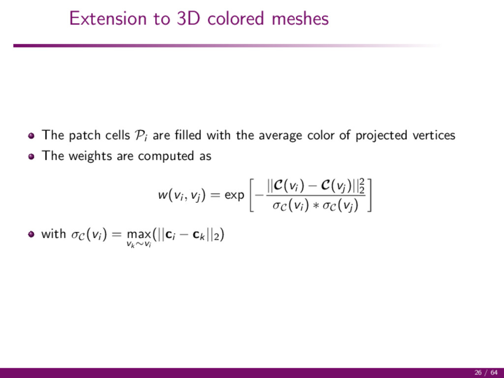
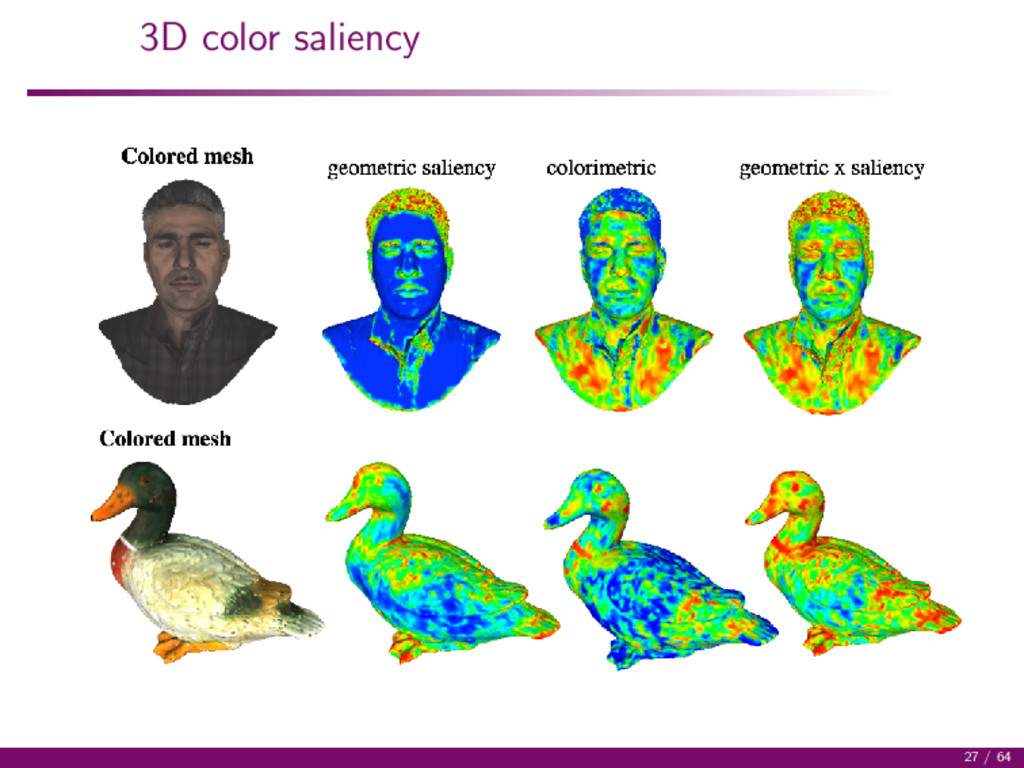
34. Extension to 3D colored meshes The patch cells Pi are filled with the average color of projected vertices The weights are computed as w(vi , vj ) = exp − ||C(vi ) − C(vj )||2 2 σC (vi ) ∗ σC (vj ) with σC (vi ) = max vk ∼vi (||ci − ck ||2 ) 26 / 64
35. 3D color saliency 27 / 64
36. 3D color saliency 27 / 64
37. 3D color saliency 27 / 64
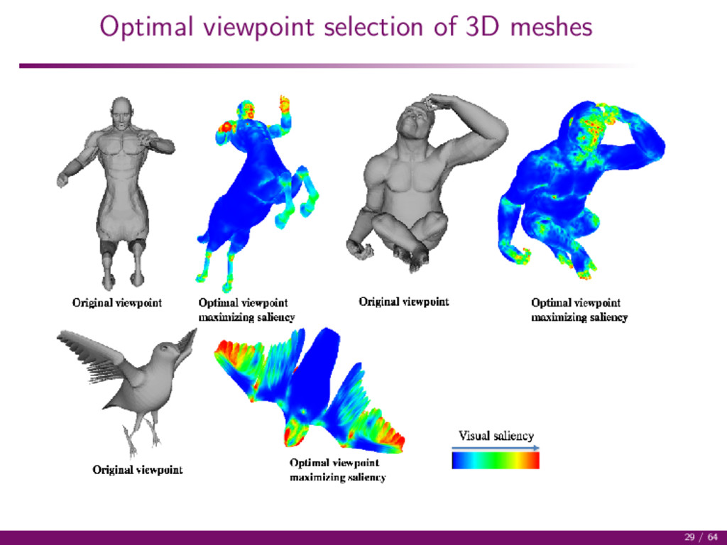
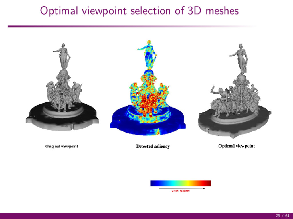
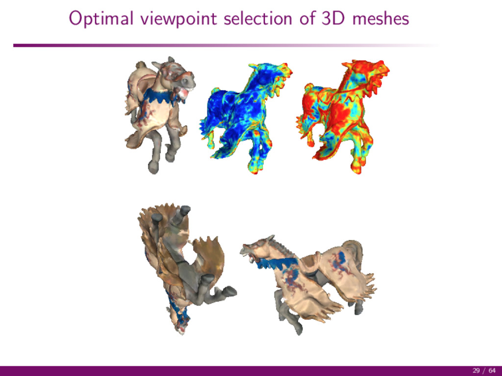
38. Optimal viewpoint selection of 3D meshes An application of saliency Goal: select viewpoints that are perceptually important for the observer Criterion: Distinguish viewpoints that maximize saliency Strategy 1 Uniformly sample a sphere bounding the 3D object 2 Select the best viewpoint VPx along the x-axis 3 From VPx, select the best viewpoint VPy along the y-axis 4 Use gradient descent from VPy in all directions 28 / 64
39. Optimal viewpoint selection of 3D meshes 29 / 64
40. Optimal viewpoint selection of 3D meshes 29 / 64
41. Optimal viewpoint selection of 3D meshes 29 / 64
42. 1 Introduction 2 3D Data Saliency 3 3D Point Cloud Colorization 4 3D Colored Mesh Enhancement 5 Conclusion 30 / 64
43. Colorization Colorization is a computer-assisted process of adding color to a monochrome image How ? The users provides example scribbles and their color is propagated in the image 31 / 64
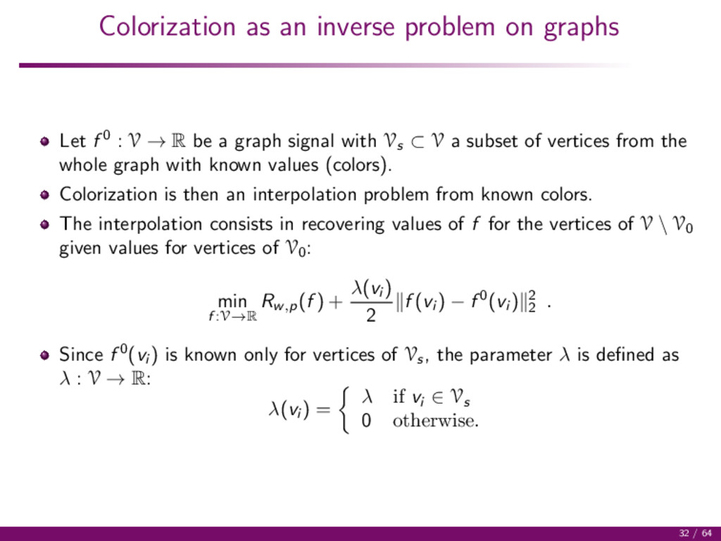
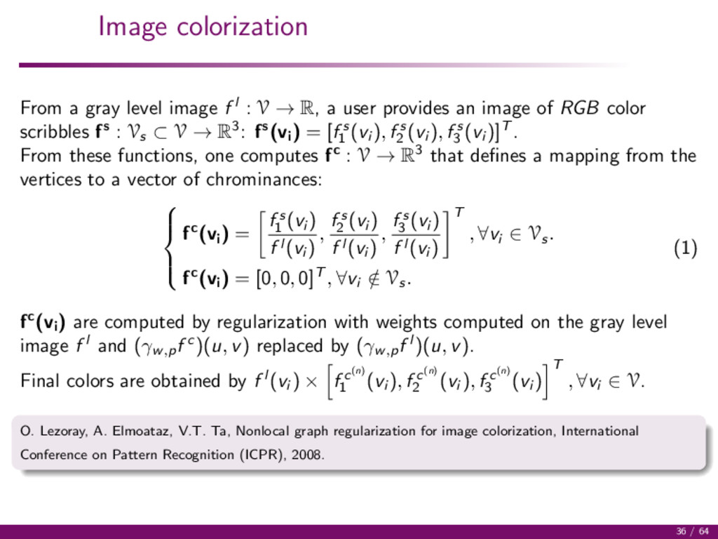
44. Colorization as an inverse problem on graphs Let f 0 : V → R be a graph signal with Vs ⊂ V a subset of vertices from the whole graph with known values (colors). Colorization is then an interpolation problem from known colors. The interpolation consists in recovering values of f for the vertices of V \ V0 given values for vertices of V0 : min f :V→R Rw,p (f ) + λ(vi ) 2 f (vi ) − f 0(vi ) 2 2 . Since f 0(vi ) is known only for vertices of Vs , the parameter λ is defined as λ : V → R: λ(vi ) = λ if vi ∈ Vs 0 otherwise. 32 / 64
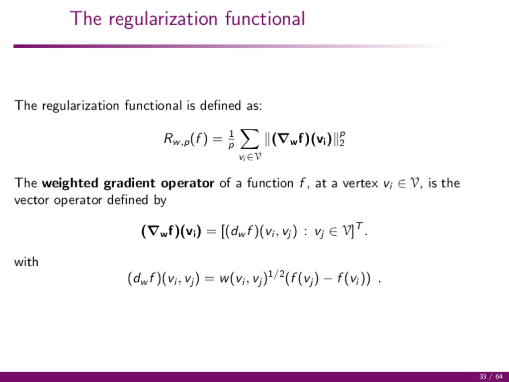
45. The regularization functional The regularization functional is defined as: Rw,p (f ) = 1 p vi ∈V (∇w f)(vi ) p 2 The weighted gradient operator of a function f , at a vertex vi ∈ V, is the vector operator defined by (∇w f)(vi ) = [(dw f )(vi , vj ) : vj ∈ V]T . with (dw f )(vi , vj ) = w(vi , vj )1/2(f (vj ) − f (vi )) . 33 / 64
46. Minimization To get the solution, we consider the following system of equations: ∂Rw,p (f ) ∂f (vi ) + λ(f (vi ) − f 0(vi )) = 0, ∀vi ∈ V. Moreover, we can prove that ∂Rw,p (f ) ∂f (vi ) = 2(∆w,p f )(vi ) with the p-Laplacian (∆w,p f )(vi ) = 1 2 vj ∼vi wij (∇w f)(vj ) p−2 2 + (∇w f)(vi ) p−2 2 (f (vi ) − f (vj )) , 34 / 64
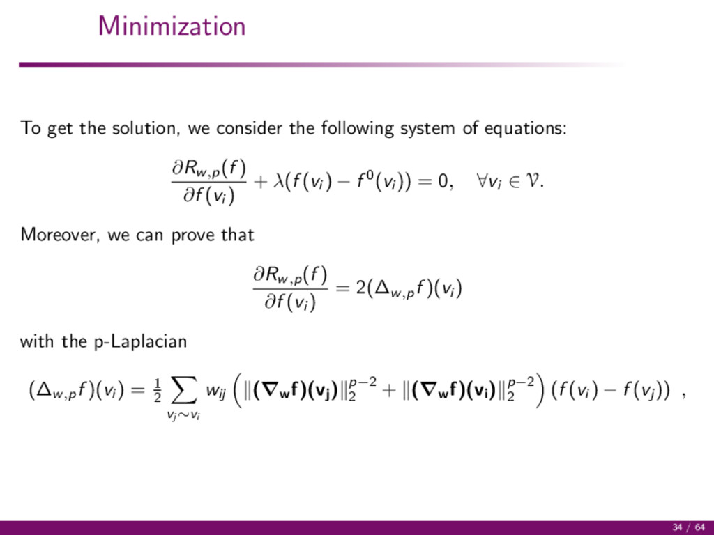
47. Minimization We use the linearized Gauss-Jacobi iterative method to solve the previous systems. Let n be an iteration step, and let f (n) be the solution at the step n. Then, the method is given by the following algorithm:        f (0) = f 0 f (n+1)(vi ) = λf 0(vi ) + vj ∼vi (γw,p f (n))(vi , vj )f (n)(vj ) λ + vj ∼vi (γw,p f (n))(vi , vj ) , ∀vi ∈ V. with (γw,p f )(vi , vj ) = wij (∇w f)(vj ) p−2 2 + (∇w f)(vi ) p−2 2 , Can be more efficiently solved using the Chambolle-Pock primal-dual algorithm (especially when p = 1). M. Hidane, O. Lezoray, A. Elmoataz, Nonlinear Multilayered Representation of Graph-Signals, Journal of Mathematical Imaging and Vision, Vol. 45(2), pp. 114-137, 2013. 35 / 64
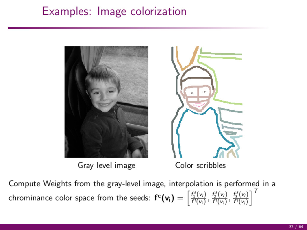
48. Image colorization From a gray level image f l : V → R, a user provides an image of RGB color scribbles fs : Vs ⊂ V → R3: fs(vi ) = [f s 1 (vi ), f s 2 (vi ), f s 3 (vi )]T . From these functions, one computes fc : V → R3 that defines a mapping from the vertices to a vector of chrominances:      fc(vi ) = f s 1 (vi ) f l (vi ) , f s 2 (vi ) f l (vi ) , f s 3 (vi ) f l (vi ) T , ∀vi ∈ Vs. fc(vi ) = [0, 0, 0]T , ∀vi / ∈ Vs. (1) fc(vi ) are computed by regularization with weights computed on the gray level image f l and (γw,p f c )(u, v) replaced by (γw,p f l )(u, v). Final colors are obtained by f l (vi ) × f c(n) 1 (vi ), f c(n) 2 (vi ), f c(n) 3 (vi ) T , ∀vi ∈ V. O. Lezoray, A. Elmoataz, V.T. Ta, Nonlocal graph regularization for image colorization, International Conference on Pattern Recognition (ICPR), 2008. 36 / 64
49. Examples: Image colorization Gray level image Color scribbles Compute Weights from the gray-level image, interpolation is performed in a chrominance color space from the seeds: fc(vi ) = f s 1 (vi ) f l (vi ) , f s 2 (vi ) f l (vi ) , f s 3 (vi ) f l (vi ) T 37 / 64
50. Examples: Image colorization p = 1, G1 , Pf0 0 = f 0 p = 1, G5 , Pf0 2 38 / 64
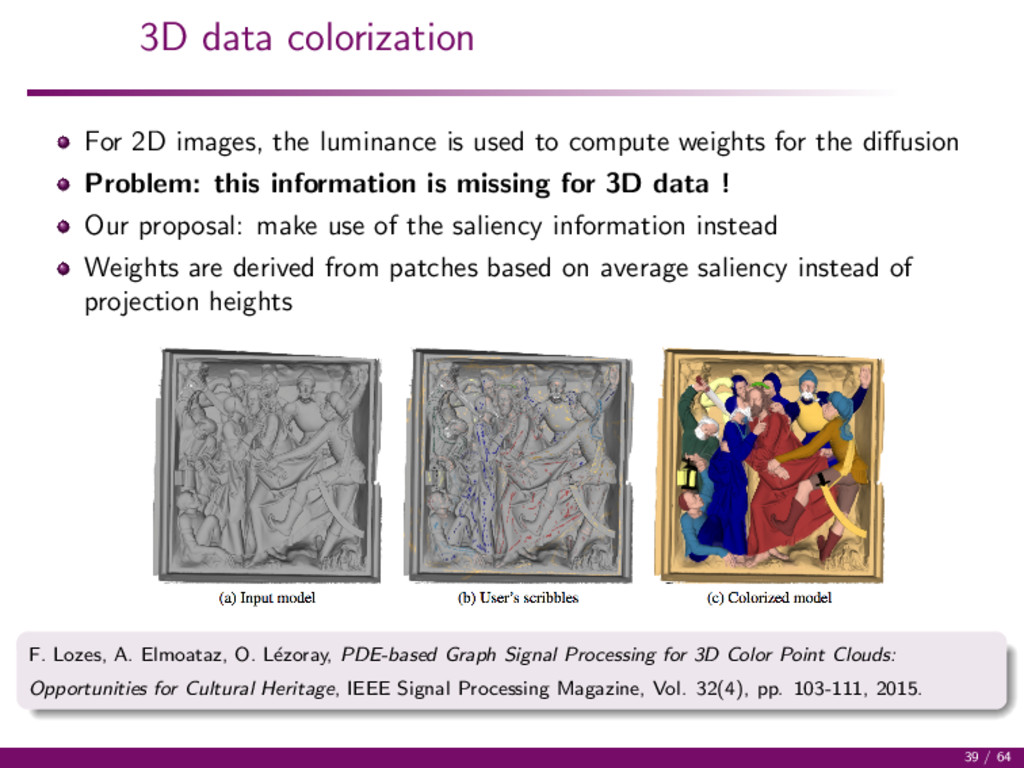
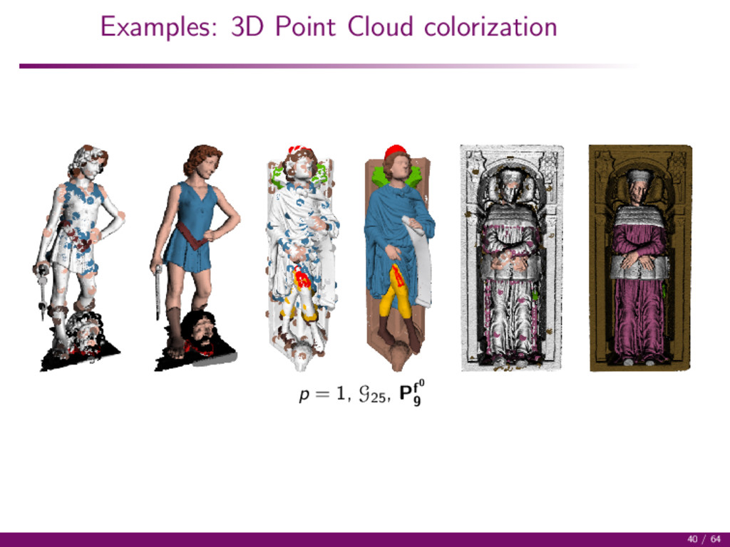
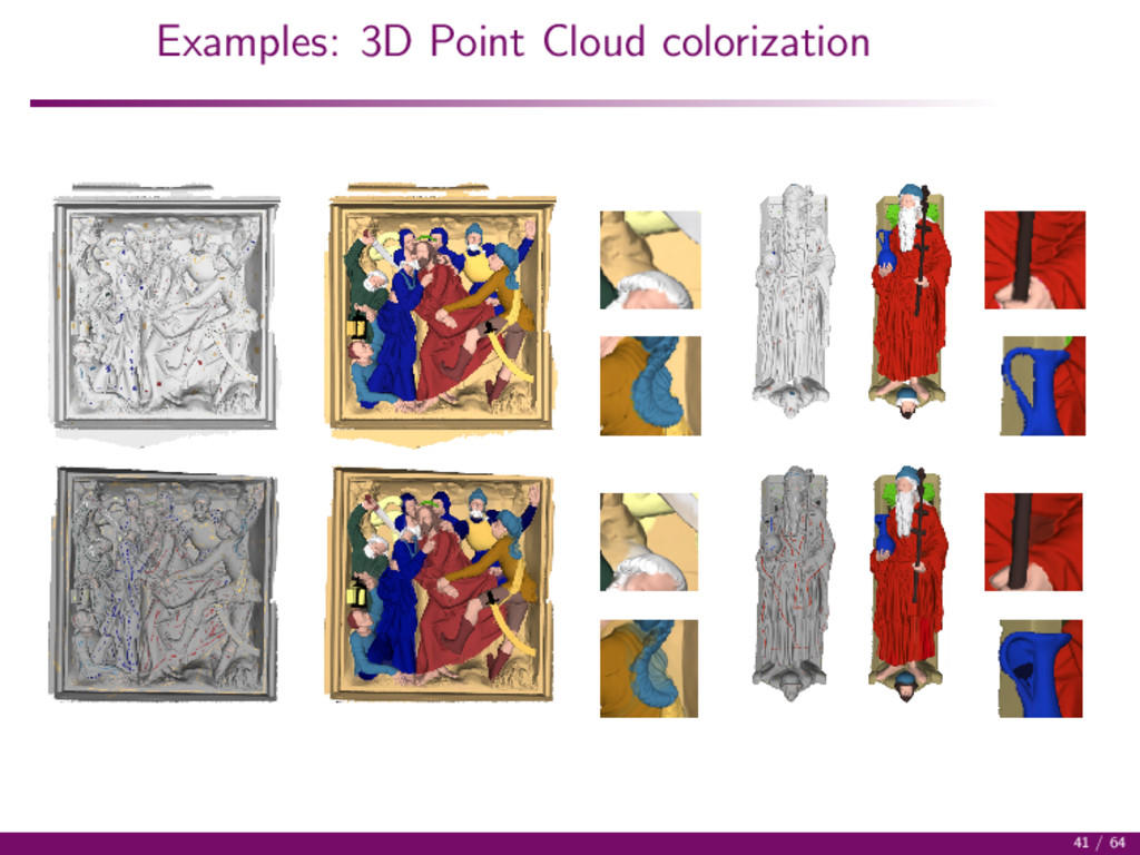
51. 3D data colorization For 2D images, the luminance is used to compute weights for the diffusion Problem: this information is missing for 3D data ! Our proposal: make use of the saliency information instead Weights are derived from patches based on average saliency instead of projection heights F. Lozes, A. Elmoataz, O. L´ ezoray, PDE-based Graph Signal Processing for 3D Color Point Clouds: Opportunities for Cultural Heritage, IEEE Signal Processing Magazine, Vol. 32(4), pp. 103-111, 2015. 39 / 64
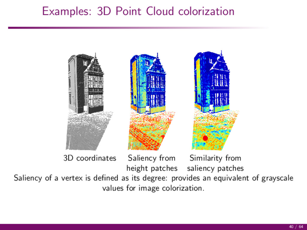
52. Examples: 3D Point Cloud colorization 3D coordinates Saliency from Similarity from height patches saliency patches Saliency of a vertex is defined as its degree: provides an equivalent of grayscale values for image colorization. 40 / 64
53. Examples: 3D Point Cloud colorization p = 1, G25 , Pf0 9 40 / 64
54. Examples: 3D Point Cloud colorization 41 / 64
55. 1 Introduction 2 3D Data Saliency 3 3D Point Cloud Colorization 4 3D Colored Mesh Enhancement 5 Conclusion 42 / 64
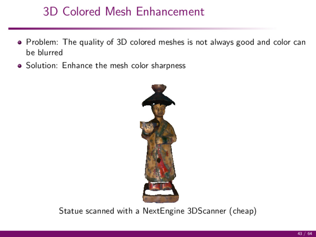
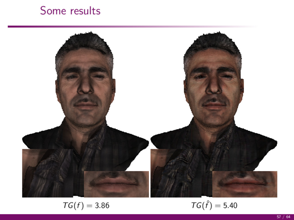
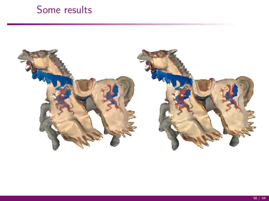
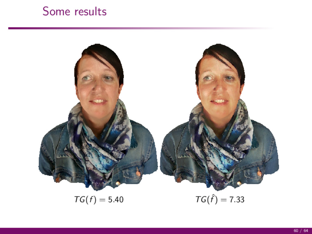
56. 3D Colored Mesh Enhancement Problem: The quality of 3D colored meshes is not always good and color can be blurred Solution: Enhance the mesh color sharpness Statue scanned with a NextEngine 3DScanner (cheap) 43 / 64
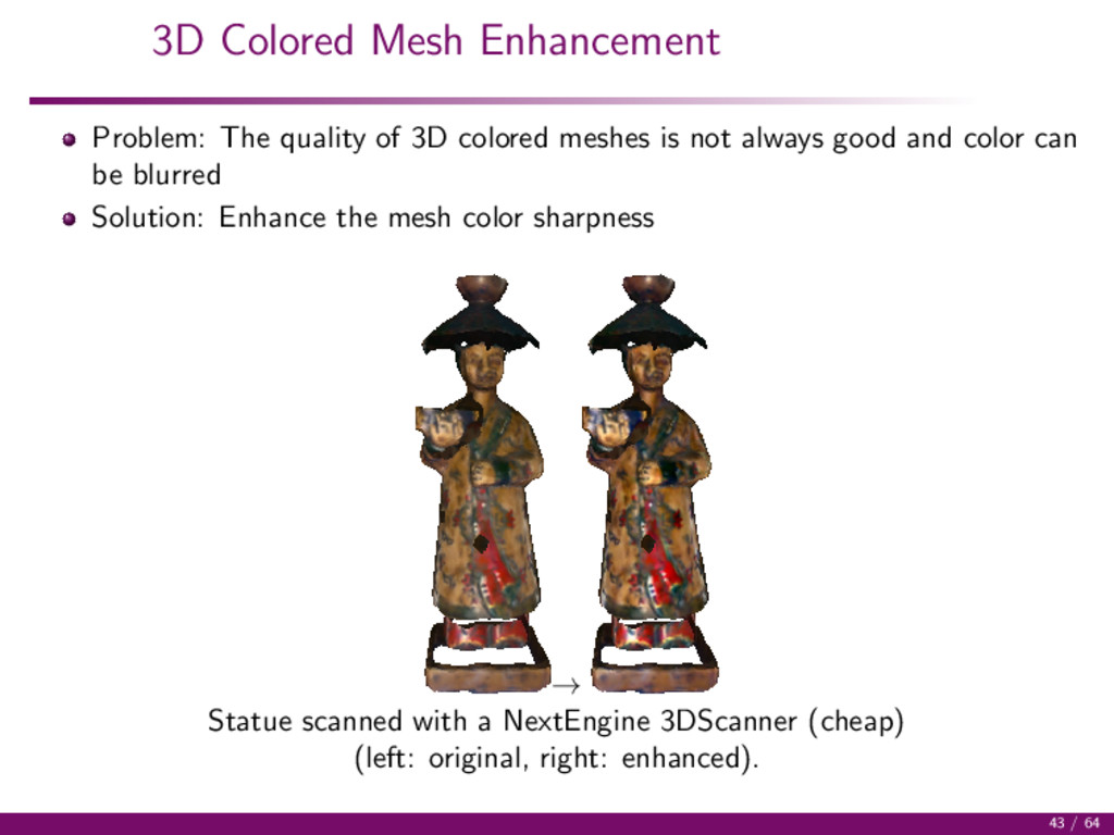
57. 3D Colored Mesh Enhancement Problem: The quality of 3D colored meshes is not always good and color can be blurred Solution: Enhance the mesh color sharpness → Statue scanned with a NextEngine 3DScanner (cheap) (left: original, right: enhanced). 43 / 64
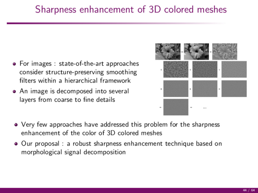
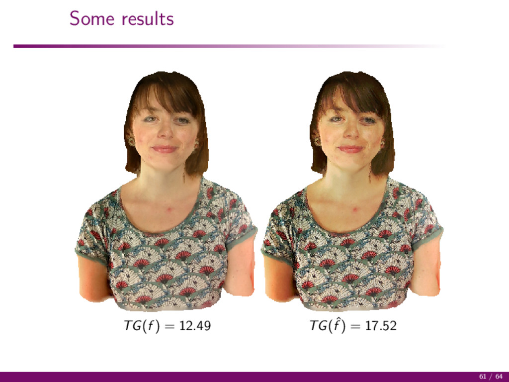
58. Sharpness enhancement of 3D colored meshes For images : state-of-the-art approaches consider structure-preserving smoothing filters within a hierarchical framework An image is decomposed into several layers from coarse to fine details Very few approaches have addressed this problem for the sharpness enhancement of the color of 3D colored meshes Our proposal : a robust sharpness enhancement technique based on morphological signal decomposition 44 / 64
59. Complete Lattice To process graph signals with mathematical morphology, we build a new signal representation in the form of an index associated with an ordering of the vectors T of an graph signal. Ordering all the values of the set T can be done with the use of an ordering relation within vectors. This amounts to dispose of a complete lattice (T , ≤) but there is no universal order for vectorial data The framework of h-orderings can be considered for that : construct a surjective mapping h from T to L where L is a complete lattice equipped with the conditional total ordering h : T → L and v → h(v), ∀(vi , vj ) ∈ T × T vi ≤h vj ⇔ h(vi ) ≤ h(vj ) . ≤h will denote such an h-ordering 45 / 64
60. Manifold-based color ordering × Problem : the projection operator h cannot be linear since a distortion of the space is inevitable ! 46 / 64
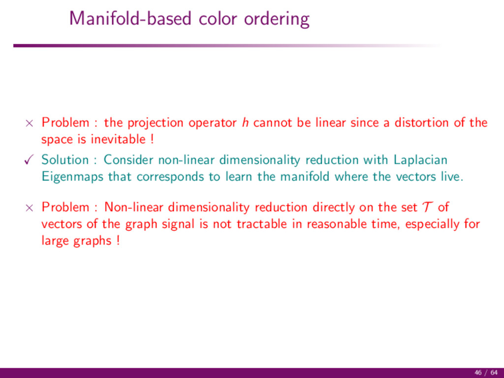
61. Manifold-based color ordering × Problem : the projection operator h cannot be linear since a distortion of the space is inevitable ! Solution : Consider non-linear dimensionality reduction with Laplacian Eigenmaps that corresponds to learn the manifold where the vectors live. 46 / 64
62. Manifold-based color ordering × Problem : the projection operator h cannot be linear since a distortion of the space is inevitable ! Solution : Consider non-linear dimensionality reduction with Laplacian Eigenmaps that corresponds to learn the manifold where the vectors live. × Problem : Non-linear dimensionality reduction directly on the set T of vectors of the graph signal is not tractable in reasonable time, especially for large graphs ! 46 / 64
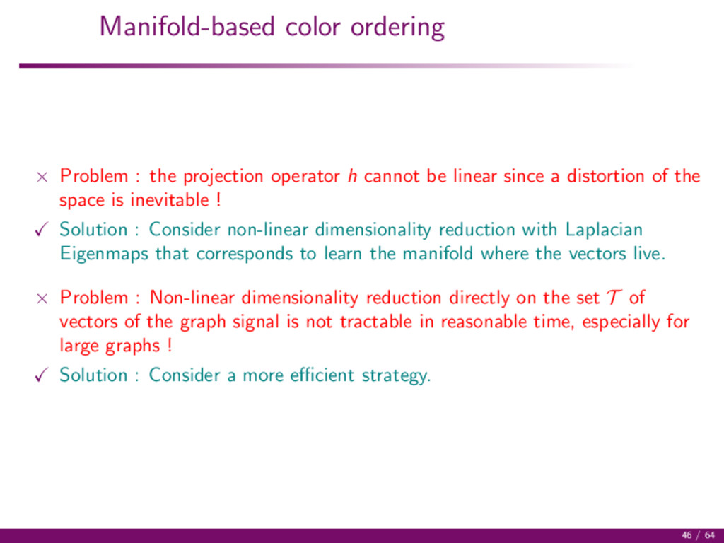
63. Manifold-based color ordering × Problem : the projection operator h cannot be linear since a distortion of the space is inevitable ! Solution : Consider non-linear dimensionality reduction with Laplacian Eigenmaps that corresponds to learn the manifold where the vectors live. × Problem : Non-linear dimensionality reduction directly on the set T of vectors of the graph signal is not tractable in reasonable time, especially for large graphs ! Solution : Consider a more efficient strategy. 46 / 64
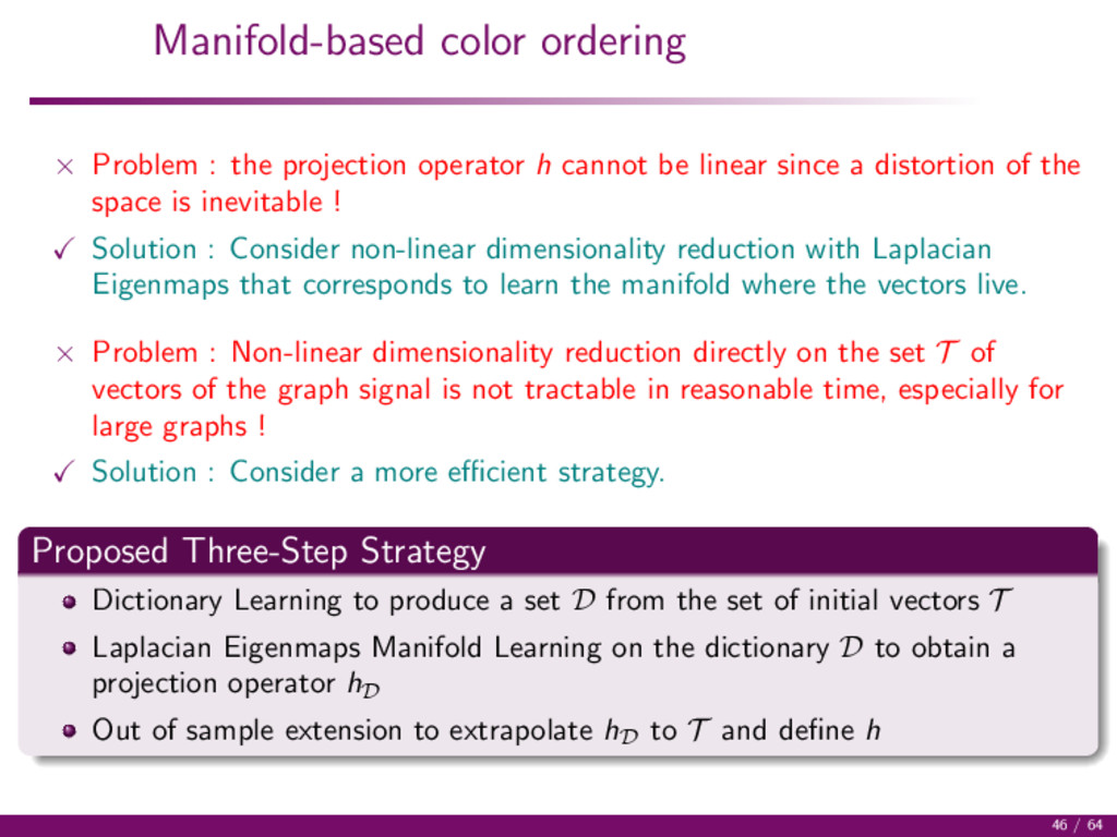
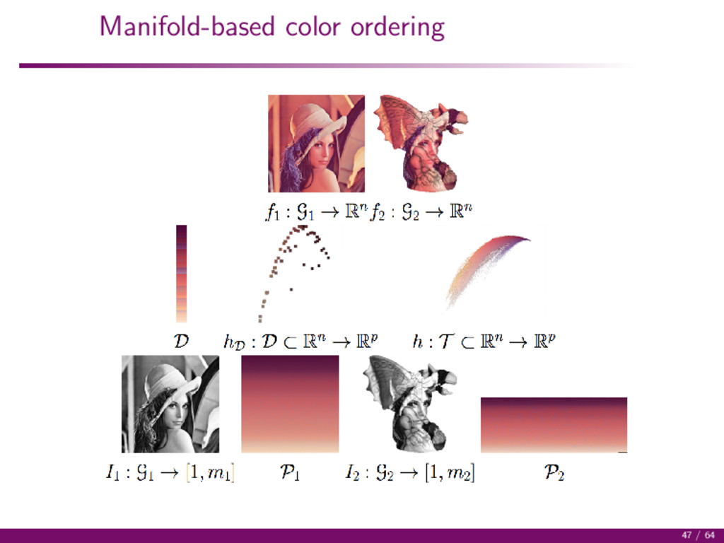
64. Manifold-based color ordering × Problem : the projection operator h cannot be linear since a distortion of the space is inevitable ! Solution : Consider non-linear dimensionality reduction with Laplacian Eigenmaps that corresponds to learn the manifold where the vectors live. × Problem : Non-linear dimensionality reduction directly on the set T of vectors of the graph signal is not tractable in reasonable time, especially for large graphs ! Solution : Consider a more efficient strategy. Proposed Three-Step Strategy Dictionary Learning to produce a set D from the set of initial vectors T Laplacian Eigenmaps Manifold Learning on the dictionary D to obtain a projection operator hD Out of sample extension to extrapolate hD to T and define h 46 / 64
65. Manifold-based color ordering 47 / 64
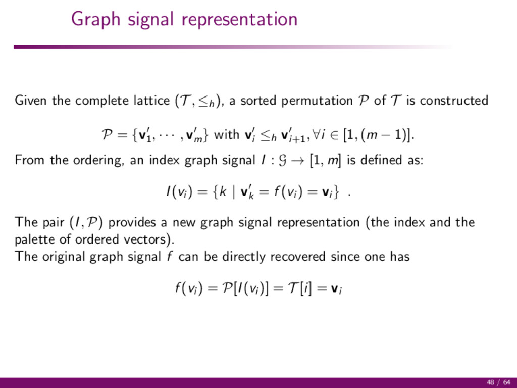
66. Graph signal representation Given the complete lattice (T , ≤h ), a sorted permutation P of T is constructed P = {v1 , · · · , vm } with vi ≤h vi+1 , ∀i ∈ [1, (m − 1)]. From the ordering, an index graph signal I : G → [1, m] is defined as: I(vi ) = {k | vk = f (vi ) = vi } . The pair (I, P) provides a new graph signal representation (the index and the palette of ordered vectors). The original graph signal f can be directly recovered since one has f (vi ) = P[I(vi )] = T [i] = vi 48 / 64
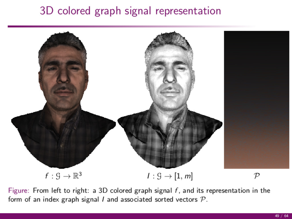
67. 3D colored graph signal representation f : G → R3 I : G → [1, m] P Figure: From left to right: a 3D colored graph signal f , and its representation in the form of an index graph signal I and associated sorted vectors P. 49 / 64
68. Graph signal morphological processing The index graph signal I can be directly used to process the original graph signal, however, to be able to reconstruct the result, the values have to be kept within [1, m]. · A processing g operating on I must be a vector preserving one : g(f (vi )) = P[g(I(vi ))] . Typical vector preserving processing operations: morphological ones. Erosion and dilation of a graph signal f at vertex vi ∈ G by a structuring element Bk ⊂ G as: Bk (f )(vi ) = {P[∧I(vj )], vj ∈ Bk (vi )} δB (f )(vi ) = {P[∨I(vj )], vj ∈ Bk (vi )} A structuring element Bk (vi ) of size k defined at a vertex vi corresponds to the set of vertices that can be reached from vi in k walks: Bk (vi ) = {vj ∼ vi } ∪ {vi } if k = 1 Bk−1 (vi ) ∪ ∪∀vl ∈Bk−1(vi ) B1 (vl ) if k ≥ 2 50 / 64
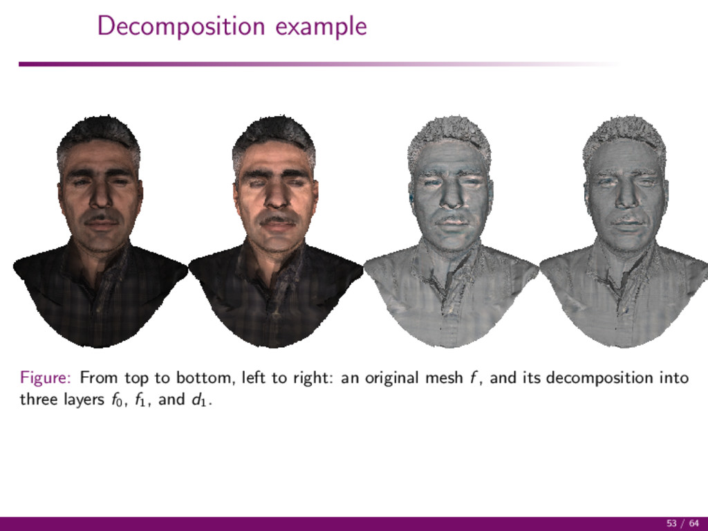
69. Graph signal multi-layer decomposition We propose the following multi-layer morphological decomposition of a graph signal into l layers. The graph signal is decomposed into a base layer and several detail layers, each capturing a given scale of details. d−1 = f , i = 0 while i < l do Compute the graph signal representation at level i − 1: di−1 = (Ii−1, Pi−1 ) Morphological Filtering of di−1 : fi = MFBl−i (di−1 ) Compute the residual (detail layer): di = di−1 − fi Proceed to next layer: i = i + 1 end while 51 / 64
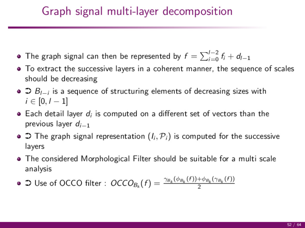
70. Graph signal multi-layer decomposition The graph signal can then be represented by f = l−2 i=0 fi + dl−1 To extract the successive layers in a coherent manner, the sequence of scales should be decreasing · Bl−i is a sequence of structuring elements of decreasing sizes with i ∈ [0, l − 1] Each detail layer di is computed on a different set of vectors than the previous layer di−1 · The graph signal representation (Ii , Pi ) is computed for the successive layers The considered Morphological Filter should be suitable for a multi scale analysis · Use of OCCO filter : OCCOBk (f ) = γBk (φBk (f ))+φBk (γBk (f )) 2 52 / 64
71. Decomposition example Figure: From top to bottom, left to right: an original mesh f , and its decomposition into three layers f0 , f1 , and d1 . 53 / 64
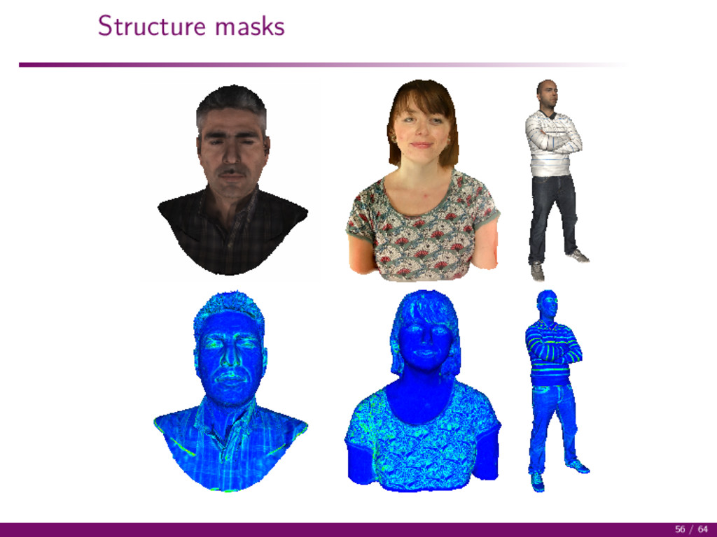
72. Graph signal enhancement The graph signal can be enhanced by manipulating the different layers with specific coefficients and adding the modified layers altogether. ˆ f (vk ) = S0 (f0 (vk )) + M(vk ) · l−1 i=1 Si (fi (vk )) with fl−1 = dl−1 (2) Each layer is manipulated by a nonlinear function Si (x) = 1 1+exp(−αi x) for detail enhancement and tone manipulation. A structure mask M prevents boosting noise and artifacts while enhancing the main structures. 54 / 64
73. Structure mask · It is preferable to boost strong structures and keep unmodified other areas. · Saliency can be considered to that aim A normalized sum of distances within a local neighborhood is a good indicator of the graph signal structure: δ(vi ) = vj ∈B1(vi ) dEMD (H(vj ), H(vi )) |B1 (vi )| (3) dEMD is the Earth Mover Distance between the color histograms within a 1-hop. Structure mask is defined as (close to 1 for constant areas and to 2 for ramp edges): M(vi ) = 1 + δ(vi ) − ∧δ ∨δ − ∧δ (4) 55 / 64
74. Structure masks 56 / 64
75. Some results TG(f ) = 3.86 TG(ˆ f ) = 5.40 57 / 64
76. Some results 58 / 64
77. Some results 59 / 64
78. Some results TG(f ) = 5.40 TG(ˆ f ) = 7.33 60 / 64
79. Some results TG(f ) = 12.49 TG(ˆ f ) = 17.52 61 / 64
80. 1 Introduction 2 3D Data Saliency 3 3D Point Cloud Colorization 4 3D Colored Mesh Enhancement 5 Conclusion 62 / 64
81. Conclusion We have proposed: A formulation of Saliency for 3D Data An application of 3D saliency for optimal point of view selection A formulation of 3D Colorization as an inverse problem on graphs, weighted by saliency A morphological decomposition of graph signals, recomposed with the use of saliency for sharpening 63 / 64
82. The end Publications available at : https://lezoray.users.greyc.fr Work funded under ANR-14-CE27-0001 GRAPHSIP and from the European Union FEDER/FSE 2014/2020 (GRAPHSIP project) 64 / 64