Population games via optimal transport

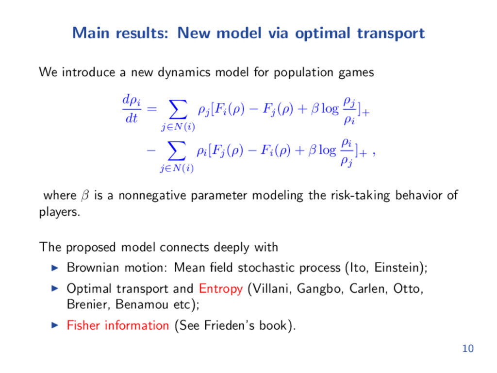
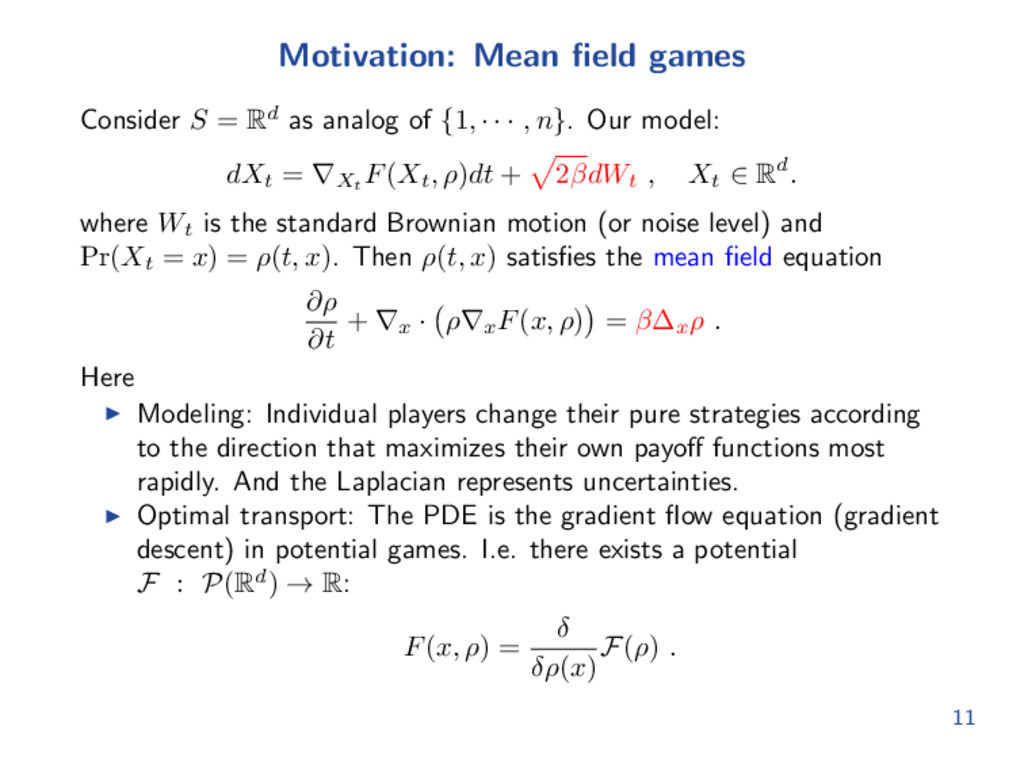
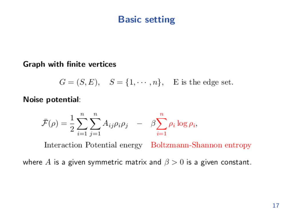
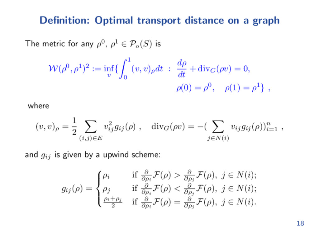
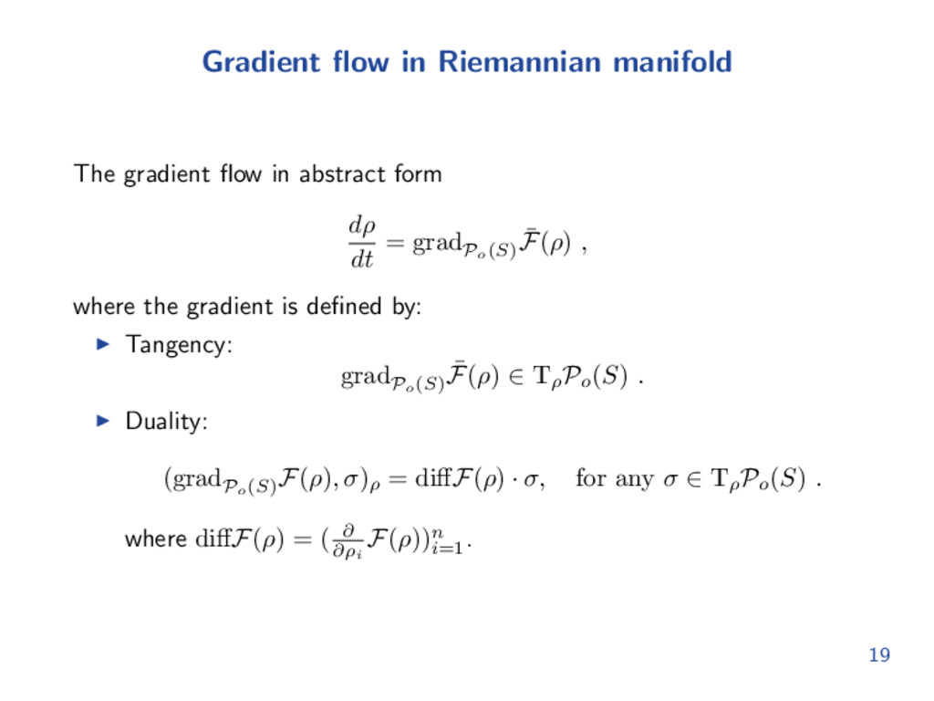
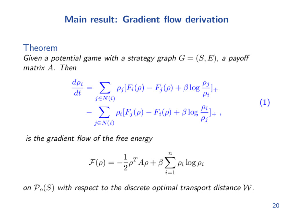
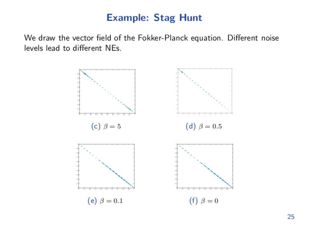
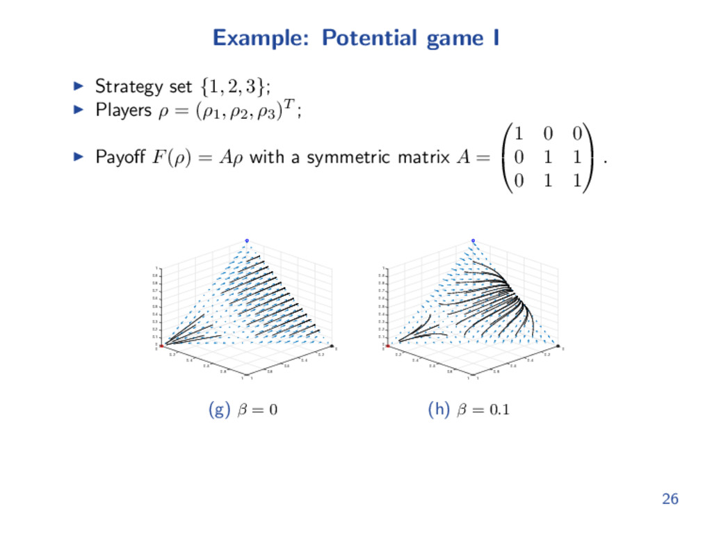
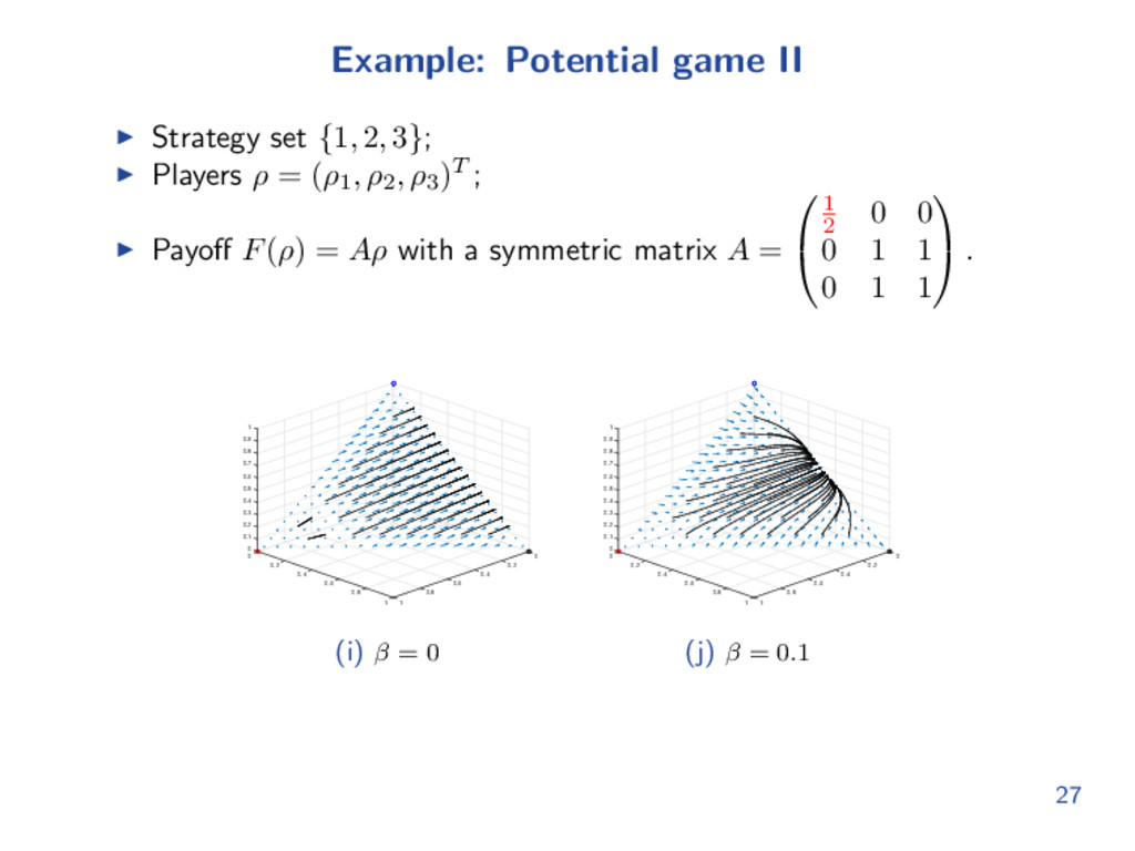
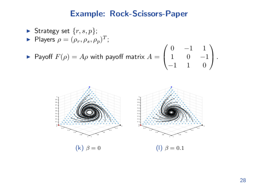
We propose a new evolutionary dynamics for population games with a discrete strategy set, inspired by the theory of optimal transport and Mean field games. The dynamics can be described as a Fokker-Planck equation on a discrete strategy set. The derived dynamics is the gradient flow of a free energy and the transition density equation of a Markov process. Such process provides models for the behavior of the individual players in population, which is myopic, greedy and irrational. The stability of the dynamics is governed by optimal transport metric, entropy and Fisher information.

Transcript

1. Population games via discrete optimal transport Wuchen Li UCLA April 28, 2017
2. Games Game contains: Players; Strategies; Payoffs. Example: Rock-Paper-Scissors game Players: 2; Strategies: S1 = S2 = {Rock, Paper, Scissors}; Payoffs: F1 , F2 : S1 × S2 → {+1, 0, −1}. 2
3. Example: Prisoner’s Dilemma 3
4. Finite players’ game Finite players’ games model the strategic interactions in N players. Player v receive a payoff depending all others Fv : S1 × · · · × SN → R ; Each player faces his/her own payoff problem: max xv∈Sv Fv (x1 , · · · , xv , · · · , xN ) , v ∈ {1, · · · , N} . People study a particular status in games, named Nash equilibrium (NE), meaning that no player has incentives to change his/her current strategy unilaterally. A strategy profile (x∗ 1 , · · · , x∗ N ) is a NE if Fv (· · · x∗ v−1 , x∗ v , x∗ v+1 , · · · ) ≥ Fv (· · · , x∗ v−1 , xv , x∗ v+1 , · · · ) , for any player v with xv ∈ Sv . 4
5. Stag hunt (Population game) Players: Infinity; Strategy set: S = {C, D}; Players form (ρC , ρD ) with ρC + ρD = 1; Payoffs: F(ρ) = (FC (ρ), FD (ρ))T = Aρ, where A = 3 0 2 2 , meaning a Deer worthing 6, a rabbit worthing 2. 5
6. Population game Population games model the strategic interactions in large populations of small, anonymous agents. It is a limiting procedure of finite players’ games. Strategy set S = {1, · · · , n} ; Players (Simplex) P(S) = {(ρi )n i=1 ∈ Rn : n i=1 ρi = 1 , ρi ≥ 0} ; Payoff function to strategy i: Fi : P(S) → R. E.g. F(ρ) = (Fi (ρ))n i=1 = Aρ , where A ∈ Rn×n . Applications Social Network, Biology species, Virus, Trading, Cancer, Congestion and many more. We plan to design new dynamics to model for the evolution of a game, and study their asymptotic properties. 6
7. Nash equilibrium and Potential games Nash Equilibrium (NE): Players have no unilateral incentive to deviate from their current strategies. ρ∗ = (ρ∗ i )n i=1 is a Nash equilibrium (NE) if ρ∗ i > 0 implies that Fi (ρ∗) ≥ Fj (ρ∗) for all j ∈ S. A particular type of game, named Potential games, are widely considered: There exists a potential F : P(S) → R, such that ∂ ∂ρi F(ρ) = Fi (ρ) . E.g. if F(ρ) = Aρ, consider F(ρ) = 1 2 ρT Aρ, where A is a symmetric matrix. In potential games, from KKT condition, NE is the critical points of max ρ F(ρ) : ρ ∈ P(S) . 7
8. Evolutionary dynamics In literature, people have designed many dynamics, named mean or evolutionary dynamics, to model games. Typical examples are BNN (Brown-von Neumann-Nash 50), Best response dynamics (Gilboa-Matsui 91), Logit (Fudenberg-Levine 98), Smith dynamics (Smith 1983) and more. One of the most widely used dynamics is Replicator dynamics (Taylor and Jonker 1978) dρi dt = ρi (Fi (ρ) − ¯ F(ρ)), where ¯ F(ρ) = j∈S ρj Fj (ρ). In potential games, the Replicator dynamics is a gradient flow in probability set P(S) w.r.t to a modified Euclidean metric (Akin (1980)). 8
9. Our Goal and Methodology Design a new dynamics for the evolutionary games to have the following properties: (i) Evolution only using local information; (ii) Locally the best choice (a gradient flow in potential games); (iii) Ability to include noise perturbations. Mathematics: Optimization; Dynamical system; Optimal transport; Riemannian Geometry; Optimal control; Partial differential equations; Graph theory; Entropy; Fisher information, etc. 9
10. Main results: New model via optimal transport We introduce a new dynamics model for population games dρi dt = j∈N(i) ρj [Fi (ρ) − Fj (ρ) + β log ρj ρi ]+ − j∈N(i) ρi [Fj (ρ) − Fi (ρ) + β log ρi ρj ]+ , where β is a nonnegative parameter modeling the risk-taking behavior of players. The proposed model connects deeply with Brownian motion: Mean field stochastic process (Ito, Einstein); Optimal transport and Entropy (Villani, Gangbo, Carlen, Otto, Brenier, Benamou etc); Fisher information (See Frieden’s book). 10
11. Motivation: Mean field games Consider S = Rd as analog of {1, · · · , n}. Our model: dXt = ∇Xt F(Xt , ρ)dt + 2βdWt , Xt ∈ Rd. where Wt is the standard Brownian motion (or noise level) and Pr(Xt = x) = ρ(t, x). Then ρ(t, x) satisfies the mean field equation ∂ρ ∂t + ∇x · ρ∇x F(x, ρ) = β∆x ρ . Here Modeling: Individual players change their pure strategies according to the direction that maximizes their own payoff functions most rapidly. And the Laplacian represents uncertainties. Optimal transport: The PDE is the gradient flow equation (gradient descent) in potential games. I.e. there exists a potential F : P(Rd) → R: F(x, ρ) = δ δρ(x) F(ρ) . 11
12. Our derivation In this talk, we will derive a similar mean field equation on a discrete strategy set. It is a gradient flow. In order to attach such a goal, we shall introduce the theory of optimal transport. 12
13. Optimal transport The problem is originally introduced by Monge in 1781, relaxed by Kantorovich by 1940 (the first example in linear programming). It introduces a particular metric on probability set, named optimal transport distance, Wasserstein metric or Earth Mover’s distance etc. 13
14. Probability Manifold In this talk, we use an important reformulation, orignated by Benamou-Breiner 2000: W(ρ0, ρ1)2 := inf v 1 0 Ev(t, Xt )2 dt , where E is the expectation operator and the infimum runs over all vector field v(t, x) with ˙ Xt = v(t, Xt ) , X0 ∼ ρ0 , X1 ∼ ρ1 . Under this metric, the probability set enjoys Riemannian geometry structures. 14
15. Gradient flow via Optimal transport The gradient flow of ¯ F(ρ) = − 1 2 Rd×Rd A(x, y)ρ(x)ρ(y)dxdy + β Rd ρ(x) log ρ(x)dx Interaction Potential energy Boltzmann-Shannon entropy w.r.t. optimal transport metric distance is: ∂ρ ∂t + ∇ · ρ∇x δ δρ(x) ¯ F(ρ) = 0 , which is exactly the mean field equation (Ambrosio, Gigli and Savare). We quote a sentence from Villani’s book (2008): The density of gradient flow is the gradient flow in density space. 15
16. Discrete optimal transport and gradient flow? Question: Can we derive a similar gradient flow in potential games on discrete strategies? Answer: Yes, we can. The gradient flow depends on the metric of probability set. We need to build a discrete optimal transport metric. 16
17. Basic setting Graph with finite vertices G = (S, E), S = {1, · · · , n}, E is the edge set. Noise potential: ¯ F(ρ) = 1 2 n i=1 n j=1 Aij ρi ρj − β n i=1 ρi log ρi , Interaction Potential energy Boltzmann-Shannon entropy where A is a given symmetric matrix and β > 0 is a given constant. 17
18. Definition: Optimal transport distance on a graph The metric for any ρ0, ρ1 ∈ Po (S) is W(ρ0, ρ1)2 := inf v { 1 0 (v, v)ρ dt : dρ dt + divG (ρv) = 0, ρ(0) = ρ0, ρ(1) = ρ1} , where (v, v)ρ = 1 2 (i,j)∈E v2 ij gij (ρ) , divG (ρv) = −( j∈N(i) vij gij (ρ))n i=1 , and gij is given by a upwind scheme: gij (ρ) =      ρi if ∂ ∂ρi F(ρ) > ∂ ∂ρj F(ρ), j ∈ N(i); ρj if ∂ ∂ρi F(ρ) < ∂ ∂ρj F(ρ), j ∈ N(i); ρi+ρj 2 if ∂ ∂ρi F(ρ) = ∂ ∂ρj F(ρ), j ∈ N(i). 18
19. Gradient flow in Riemannian manifold The gradient flow in abstract form dρ dt = gradPo(S) ¯ F(ρ) , where the gradient is defined by: Tangency: gradPo(S) ¯ F(ρ) ∈ Tρ Po (S) . Duality: (gradPo(S) F(ρ), σ)ρ = diffF(ρ) · σ, for any σ ∈ Tρ Po (S) . where diffF(ρ) = ( ∂ ∂ρi F(ρ))n i=1 . 19
20. Main result: Gradient flow derivation Theorem Given a potential game with a strategy graph G = (S, E), a payoff matrix A. Then dρi dt = j∈N(i) ρj [Fi (ρ) − Fj (ρ) + β log ρj ρi ]+ − j∈N(i) ρi [Fj (ρ) − Fi (ρ) + β log ρi ρj ]+ , (1) is the gradient flow of the free energy F(ρ) = − 1 2 ρT Aρ + β n i=1 ρi log ρi on Po (S) with respect to the discrete optimal transport distance W. 20
21. Main result: Gradient flow Asymptotical behavior Theorem For any initial condition ρ0 ∈ Po (S), (1) has a unique solution ρ(t) : [0, ∞) → Po (S). (i) The free energy F(ρ) is a Lyapunov function of (1): (ii) If limt→∞ ρ(t) exists, call it ρ∞, then ρ∞ is one of the possible Gibbs measures, i.e. ρ∞ i = 1 K eFi(ρ∞) β , K = n i=1 eFi(ρ∞) β for all i ∈ S. 21
22. Main result: Converge of Gradient flow Theorem (Entropy dissipation) If the Gibbs measure ρ∞ is a strict maximizer of ¯ F(ρ), then there exists a constant C > 0, such that ¯ F(ρ∞) − ¯ F(ρ(t)) ≤ e−Ct( ¯ F(ρ∞) − ¯ F(ρ0)) . The exponential convergence is naturally expected because (1) is the gradient flow on a Riemannian manifold (Po (S), W). Its proof is based on the relation between entropy, Fisher information, and optimal transport metric on a graph. 22
23. Modeling: Nonlinear Markov process Let ρi (t) = Pr(Xβ (t) = i). Then ρ(t) governs the following discrete state Markov process Xβ (t): P(Xβ (t + h) = j | Xβ (t) = i) =      ( ¯ Fj (ρ) − ¯ Fi (ρ))+ h, if j ∈ N(i); 1 − j∈N(i) ( ¯ Fj (ρ) − ¯ Fi (ρ))+ h + o(h), if j ∈ N(i); 0, otherwise, where limh→0 o(h) h = 0 and ¯ Fi (ρ) = Fi (ρ) − β log ρi . 23
24. Example: Stag Hunt Strategy set {C, D}; Players ρ = (ρC , ρD )T ; Payoff F(ρ) = Aρ with A = 3 0 2 2 . 24
25. Example: Stag Hunt We draw the vector field of the Fokker-Planck equation. Different noise levels lead to different NEs. 0 0.1 0.2 0.3 0.4 0.5 0.6 0.7 0.8 0.9 1 0 0.1 0.2 0.3 0.4 0.5 0.6 0.7 0.8 0.9 1 (c) β = 5 0 0.1 0.2 0.3 0.4 0.5 0.6 0.7 0.8 0.9 1 0 0.1 0.2 0.3 0.4 0.5 0.6 0.7 0.8 0.9 1 (d) β = 0.5 0 0.1 0.2 0.3 0.4 0.5 0.6 0.7 0.8 0.9 1 0 0.1 0.2 0.3 0.4 0.5 0.6 0.7 0.8 0.9 1 (e) β = 0.1 0 0.1 0.2 0.3 0.4 0.5 0.6 0.7 0.8 0.9 1 0 0.1 0.2 0.3 0.4 0.5 0.6 0.7 0.8 0.9 1 (f) β = 0 25
26. Example: Potential game I Strategy set {1, 2, 3}; Players ρ = (ρ1 , ρ2 , ρ3 )T ; Payoff F(ρ) = Aρ with a symmetric matrix A =   1 0 0 0 1 1 0 1 1   . 0 0.2 0.4 0.6 0.8 1 1 0.8 0.6 0.4 0.2 0 0.1 0.2 0.3 0.4 0.5 0.6 0.7 0.8 0.9 1 0 (g) β = 0 0 0.2 0.4 0.6 0.8 1 1 0.8 0.6 0.4 0.2 0 0.1 0.2 0.3 0.4 0.5 1 0.9 0.8 0.7 0.6 0 (h) β = 0.1 26
27. Example: Potential game II Strategy set {1, 2, 3}; Players ρ = (ρ1 , ρ2 , ρ3 )T ; Payoff F(ρ) = Aρ with a symmetric matrix A =   1 2 0 0 0 1 1 0 1 1   . 0 0.2 0.4 0.6 0.8 1 1 0.8 0.6 0.4 0.2 0 0.1 0.2 0.3 0.4 0.5 0.6 0.7 0.8 0.9 1 0 (i) β = 0 0 0.2 0.4 0.6 0.8 1 1 0.8 0.6 0.4 0.2 0.6 0.7 0.8 0.9 1 0.5 0.4 0.3 0.2 0.1 0 0 (j) β = 0.1 27
28. Example: Rock-Scissors-Paper Strategy set {r, s, p}; Players ρ = (ρr , ρs , ρp )T ; Payoff F(ρ) = Aρ with payoff matrix A =   0 −1 1 1 0 −1 −1 1 0   . 0 0.2 0.4 0.6 0.8 1 1 0.8 0.6 0.4 0.2 0.1 0.2 0.3 0.4 0.5 0.6 0.7 0.8 0.9 1 0 0 (k) β = 0 0 0.2 0.4 0.6 0.8 1 1 0.8 0.6 0.4 0.2 1 0.9 0.8 0.7 0.6 0.5 0.4 0.3 0.2 0.1 0 0 (l) β = 0.1 28
29. Example: Bad Rock-Scissors-Paper Payoff F(ρ) = Aρ with payoff matrix A =   0 −2 1 1 0 −2 −2 1 0   . We demonstrate a Hopf Bifurcation. If β is large, there is a unique equilibrium around (1 3 , 1 3 , 1 3 ). If β is small, a limit cycle exists. 0 0.2 0.4 0.6 0.8 1 1 0.8 0.6 0.4 0.2 0 0.1 0.2 1 0.9 0.8 0.7 0.6 0.5 0.4 0.3 0 (m) β = 0.5 0 0.2 0.4 0.6 0.8 1 1 0.8 0.6 0.4 0.2 1 0 0.1 0.2 0.3 0.4 0.5 0.6 0.7 0.8 0.9 0 (n) β = 0.1 0 0.2 0.4 0.6 0.8 1 1 0.8 0.6 0.4 0.2 0.1 0.2 0.5 0 0.3 0.4 1 0.9 0.8 0.7 0.6 0 (o) β = 0 29
30. Conclusion The new model has some desirable properties: It is the gradient flow of the noisy potential in the probability space endowed with the optimal transport metric. It is the probability evolution equation of a Markov process, which model players myopicity, greediness and irrationality. For potential games, its asymptotic properties are obtained by the relation of optimal transport metric, entropy and Fisher information. 30
31. B. Frieden Science from Fisher Information: A Unification, 2004. Wuchen Li, Penghang Yin and Stanley Osher Computations of optimal transport distance with Fisher information regularization, 2017. Shui-Nee Chow, Wuchen Li, Jun Lu and Haomin Zhou Population games and discrete optimal transport, 2017. Shui-Nee Chow, Wuchen Li and Haomin Zhou Optimal transport on finite graphs: Entropy dissipation, 2016. Wuchen Li A study of stochastic differential equation and Fokker-Planck equation with applications, Phd thesis, 2016. D. Monderer and L. Shapely, Potential games, 1996. C´ edric Villani Optimal transport: Old and new, 2008. 31
32. Thanks! 31