Onia P&P meeting 17.01.2014

Preliminary results

Transcript

1. Study of χb production at √ s =7 and 8 TeV Onia P&P meeting Sasha Mazurov University of Ferrara (Italy) & CERN 17 January 2014 1/34
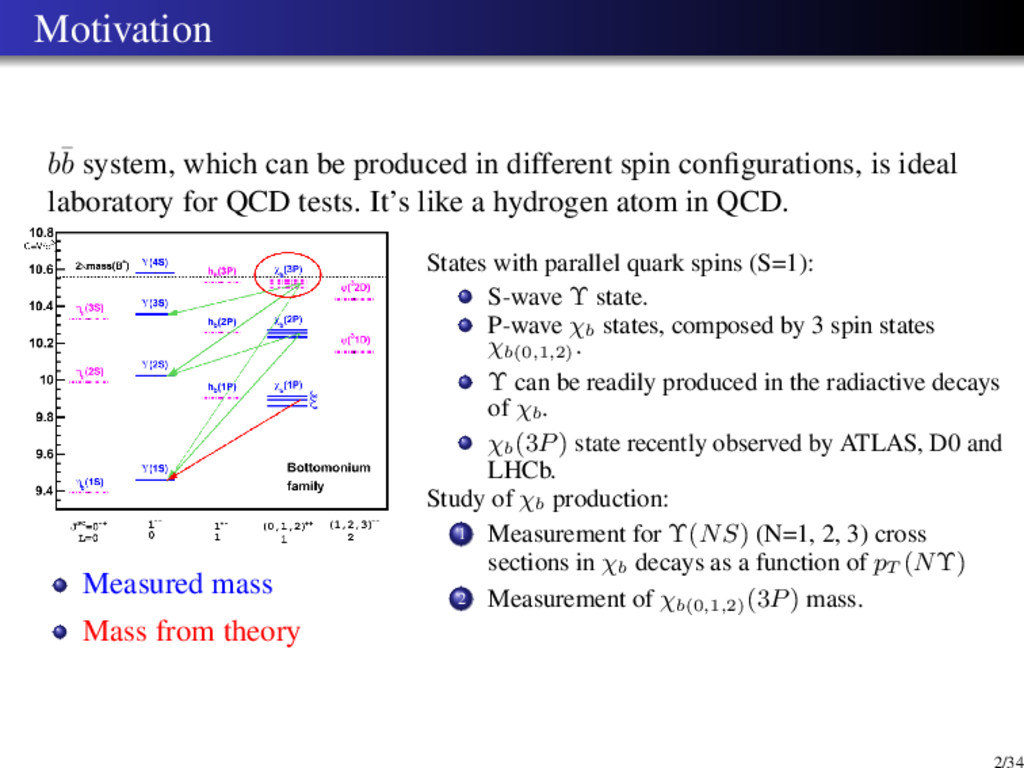
2. Motivation b¯ b system, which can be produced in different spin configurations, is ideal laboratory for QCD tests. It’s like a hydrogen atom in QCD. Measured mass Mass from theory States with parallel quark spins (S=1): S-wave Υ state. P-wave χb states, composed by 3 spin states χb(0,1,2) . Υ can be readily produced in the radiactive decays of χb. χb (3P) state recently observed by ATLAS, D0 and LHCb. Study of χb production: 1 Measurement for Υ(NS) (N=1, 2, 3) cross sections in χb decays as a function of pT (NΥ) 2 Measurement of χb(0,1,2) (3P) mass. 2/34
3. Previous analysis at LHCb ”Measurement of the fraction of Υ(1S) originating from χb(1P) in pp collisions at √ s =7 TeV ”, arXiv:1209.0282, L = 32 pb−1 ”Observation of the χb(3P) state at LHCb in pp collisions at √ s =7 TeV ”, LHCb-CONF-2012-020, L = 0.9 fb−1. 3/34
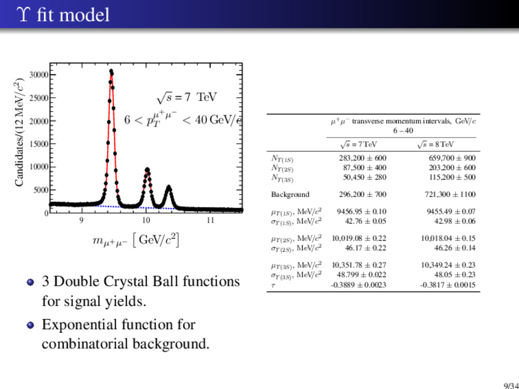
4. Cross sections formula In each pT (Υ) bin calculate: σ(χb→Υγ) σ(Υ) → Nχb→Υγ NΥ × Υ χb→Υγ = Nχb→Υγ NΥ × 1 reco γ Calculate for each Υ(nS), n = 1, 2, 3 and χb(mP), m = 1, 2, 3 Get N from fits: NΥ from m(µ+µ−) and Nχb→Υγ from [m(µ+µ−γ) − m(µ+µ−)] (for better resolution) Compute efficiency from Monte-Carlo simulation 4/34
5. Plan 1 Datasets 2 Determination of Υ yields. Fit model with double CrystalBall. 3 Determination of χb yields in the following decays χb (1, 2, 3P) → Υ(1S)γ χb (2, 3P) → Υ(2S)γ χb (3P) → Υ(3S)γ 4 Monte-Carlo efficiencies 5 Systematic uncertainties 6 Results 5/34
6. Datasets Full 2011 dataset at √ s =7 TeV. L = 1 fb−1 Full 2012 dataset at √ s =8 TeV. L = 2 fb−1 Monte-Carlo simulation of χb inclusive decays, generated 62 × 106 events. 6/34
7. The Υ selection Description Requirement Track fit quality χ2/ndf < 4 Track pT > 1 GeV/c Primary vertex probability > 0.5% Luminous region |zPV | < 0.5m and x2 PV + y2 PV < 100mm2 Kullback-Leibler distance > 5000 Muon and hadron hypotheses ∆ log Lµ−h > 0 Muon probability ProbNN > 0.5 Trigger lines: L0 DiMuon.*Decision HLT1 Hlt1DiMuonHighMass.*Decision HLT2 HLT2DiMuonB.*Decision 7/34
8. Monte-Carlo Υ Fit 9.2 9.3 9.4 9.5 9.6 9.7 0 200 400 600 800 1000 1200 1400 1600 1800 2000 -8 -6 -4 -2 0 2 4 6 Events/(5 MeV/c2) mµ+µ− GeV/c2 18 < pµ+µ− T < 22 GeV/c CrystalBall 9.2 9.3 9.4 9.5 9.6 9.7 0 200 400 600 800 1000 1200 1400 1600 1800 2000 -4 -2 0 2 4 Events/(5 MeV/c2) mµ+µ− GeV/c2 18 < pµ+µ− T < 22 GeV/c Double CrystalBall Double CrystalBall describes the Υ signal better then single CrystalBall. In data fits the following parameters are fixed: αL = 1.6, nL = 4, αR = 0.6, nR = 10. Notable improvement of χ2/n.d.f, but yields does not change so much. 8/34
9. Υ fit model 9 10 11 0 5000 10000 15000 20000 25000 30000 Candidates/(12 MeV/c2) mµ+µ− GeV/c2 √ s = 7 TeV 6 < pµ+µ− T < 40 GeV/c 3 Double Crystal Ball functions for signal yields. Exponential function for combinatorial background. µ+µ− transverse momentum intervals, GeV/c 6 – 40 √ s = 7 TeV √ s = 8 TeV NΥ(1S) 283,200 ± 600 659,700 ± 900 NΥ(2S) 87,500 ± 400 203,200 ± 600 NΥ(3S) 50,450 ± 280 115,200 ± 500 Background 296,200 ± 700 721,300 ± 1100 µΥ(1S) , MeV/c2 9456.95 ± 0.10 9455.49 ± 0.07 σΥ(1S) , MeV/c2 42.76 ± 0.05 42.98 ± 0.06 µΥ(2S) , MeV/c2 10,019.08 ± 0.22 10,018.04 ± 0.15 σΥ(2S) , MeV/c2 46.17 ± 0.22 46.26 ± 0.14 µΥ(3S) , MeV/c2 10,351.78 ± 0.27 10,349.24 ± 0.23 σΥ(3S) , MeV/c2 48.799 ± 0.022 48.05 ± 0.23 τ -0.3889 ± 0.0023 -0.3817 ± 0.0015 9/34
10. Υ masses in data fits 10 20 30 40 9.454 9.455 9.456 9.457 9.458 9.459 9.46 9.461 9.462 9.463 9.464 Υ(1S) mass GeV/c2 pµ+µ− T GeV/c2 10 20 30 40 10.015 10.016 10.017 10.018 10.019 10.02 10.021 10.022 10.023 10.024 10.025 Υ(2S) mass GeV/c2 pµ+µ− T GeV/c2 10 20 30 40 10.348 10.349 10.35 10.351 10.352 10.353 10.354 10.355 10.356 10.357 10.358 Υ(3S) mass GeV/c2 pµ+µ− T GeV/c2 √ s =7 TeV, √ s =8 TeV Υ masses is about 5 MeV/c2 lower than PDG values (dash lines). Momentum scaling correction was applied. 10/34
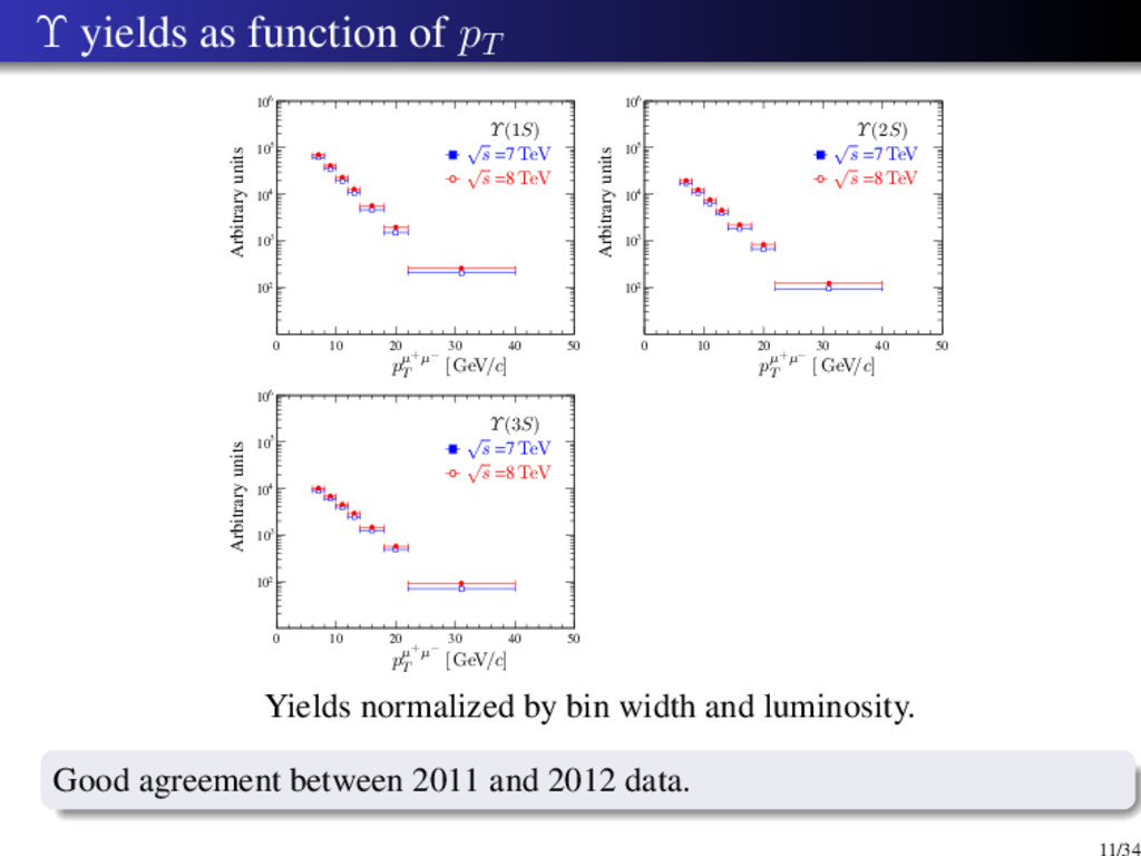
11. Υ yields as function of pT 0 10 20 30 40 50 2 10 3 10 4 10 5 10 6 10 0 10 20 30 40 50 2 10 3 10 4 10 5 10 6 10 0 10 20 30 40 50 2 10 3 10 4 10 5 10 6 10 Arbitrary units pµ+µ− T [ GeV/c] Υ(3S) Arbitrary units pµ+µ− T [ GeV/c] Υ(1S) Arbitrary units pµ+µ− T [ GeV/c] Υ(2S) √ s =7 TeV √ s =8 TeV √ s =7 TeV √ s =8 TeV √ s =7 TeV √ s =8 TeV Yields normalized by bin width and luminosity. Good agreement between 2011 and 2012 data. 11/34
12. χb selection In this study photons reconstructed using the calorimeter information. Another approach is to track e+e− (converted photons) — this method has better invariant mass resolution, but requires more statistics. Cuts on γ: Transverse momentum of γ pT (γ) > 600 MeV/c Polar angle of γ in the µ+µ−γ rest frame cos θγ > 0 Confidence level of γ cl(γ) > 0.01 Dimuon mass windows: Decay Cut Description χb(1, 2, 3P) → Υ(1S) 9310 < µ+µ− < 9600 MeV/c 3σΥ(1S) < µ+µ− < 2.5σΥ(1S) MeV/c χb(2, 3P) → Υ(2S) 9870 < µ+µ− < 10090 MeV/c 3σΥ(2S) < µ+µ− < σΥ(2S) MeV/c χb(3P) → Υ(3S) 10300 < µ+µ− < 10526 MeV/c σΥ(3S) < µ+µ− < 3σΥ(3S) MeV/c 12/34
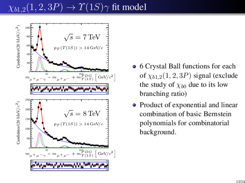
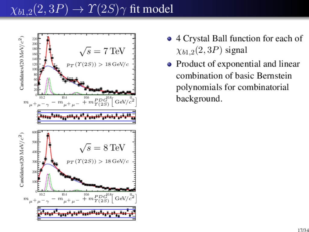
13. χb1,2 (1, 2, 3P) → Υ(1S)γ fit model 10 10.5 0 500 1000 1500 2000 2500 -4 -2 0 2 4 10 10.5 0 200 400 600 800 1000 -4 -2 0 2 4 Candidates/(20 MeV/c2) m µ+µ−γ − m µ+µ− + mP DG Υ (1S) GeV/c2 √ s = 8 TeV pT (Υ (1S)) > 14 GeV/c Candidates/(20 MeV/c2) m µ+µ−γ − m µ+µ− + mP DG Υ (1S) GeV/c2 √ s = 7 TeV pT (Υ (1S)) > 14 GeV/c 6 Crystal Ball functions for each of χb1,2(1, 2, 3P) signal (exclude the study of χb0 due to its low branching ratio) Product of exponential and linear combination of basic Bernstein polynomials for combinatorial background. 13/34
14. χb1,2 (1, 2, 3P) → Υ(1S)γ fit model (2) Free parameters: µχb1(1P), yields and background parameters. Linked parameters for χb1 and χb2 signals: µχb2(jP ) = µχb1(jP ) + ∆mP DG χb2(jP ) , j=1,2 µχb2(3P ) = µχb1(3P ) + ∆mtheory χb2(3P ) Nχb = λNχb1 + (1 − λ)Nχb2 σχb2 = σχb1 Other linked parameters: µχb1(2P ) = µχb1(1P ) + ∆mP DG χb1(2P ) µχb1(3P ) = µχb1(1P ) + ∆mχb1(3P ) (∆mχb1(3P ) measured in this study) Fixed parameters from MC study: σχb1(1P ) scaled by 1.17, σχb1(2P ) σχb1(1P ) , σχb1(3P ) σχb1(1P ) α and n parameters of CB. Υ(1S) transverse momentum intervals, GeV/c 14 — 40 √ s = 7 TeV √ s = 8 TeV Nχb(1P) 2090 ± 80 5150 ± 130 Nχb(2P) 450 ± 50 1030 ± 100 Nχb(3P) 160 ± 40 230 ± 50 Background 8820 ± 130 23,800 ± 200 µχb1(1P) , MeV/c 9889.7 ± 1.0 9890.3 ± 0.7 σχb1(1P) , MeV/c 22.0 23.2 τ -2.6 ± 0.5 -3.29 ± 0.33 c1 -0.09 ± 0.12 0.07 ± 0.07 c2 1.33 ± 0.04 0.296 ± 0.023 χ2/n.d.f 1.03 1.24 14/34
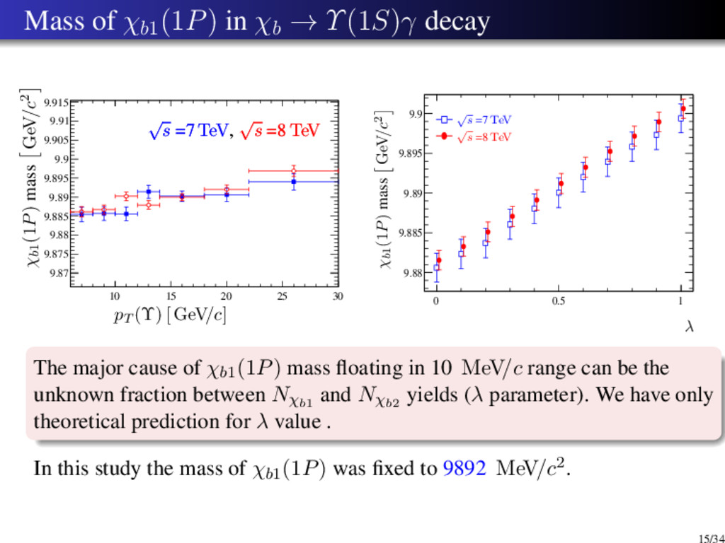
15. Mass of χb1 (1P) in χb → Υ(1S)γ decay 10 15 20 25 30 9.87 9.875 9.88 9.885 9.89 9.895 9.9 9.905 9.91 9.915 √ s =7 TeV, √ s =8 TeV √ s =7 TeV, √ s =8 TeV χb1(1P) mass GeV/c2 pT (Υ) [ GeV/c] 0 0.5 1 9.88 9.885 9.89 9.895 9.9 χb1(1P) mass GeV/c2 λ √ s =7 TeV √ s =8 TeV The major cause of χb1(1P) mass floating in 10 MeV/c range can be the unknown fraction between Nχb1 and Nχb2 yields (λ parameter). We have only theoretical prediction for λ value . In this study the mass of χb1(1P) was fixed to 9892 MeV/c2. 15/34
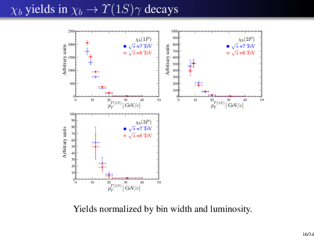
16. χb yields in χb → Υ(1S)γ decays 0 10 20 30 40 50 0 10 20 30 40 50 60 70 80 90 100 0 10 20 30 40 50 0 500 1000 1500 2000 2500 0 10 20 30 40 50 0 100 200 300 400 500 600 700 800 900 1000 Arbitrary units pΥ(1S) T [ GeV/c] χb(3P) Arbitrary units pΥ(1S) T [ GeV/c] χb(1P) Arbitrary units pΥ(1S) T [ GeV/c] χb(2P) √ s =7 TeV √ s =8 TeV √ s =7 TeV √ s =8 TeV √ s =7 TeV √ s =8 TeV Yields normalized by bin width and luminosity. 16/34
17. χb1,2 (2, 3P) → Υ(2S)γ fit model 10.2 10.4 10.6 10.8 11 0 100 200 300 400 500 600 -4 -2 0 2 4 10.2 10.4 10.6 10.8 11 0 20 40 60 80 100 120 140 160 180 200 220 -4 -2 0 2 4 Candidates/(20 MeV/c2) m µ+µ−γ − m µ+µ− + mP DG Υ (2S) GeV/c2 √ s = 8 TeV pT (Υ (2S)) > 18 GeV/c Candidates/(20 MeV/c2) m µ+µ−γ − m µ+µ− + mP DG Υ (2S) GeV/c2 √ s = 7 TeV pT (Υ (2S)) > 18 GeV/c 4 Crystal Ball function for each of χb1,2(2, 3P) signal Product of exponential and linear combination of basic Bernstein polynomials for combinatorial background. 17/34
18. χb1,2 (2, 3P) → Υ(2S)γ fit model (2) Free parameters: µχb1(2P), yields and background parameters. Linked parameters for χb1 and χb2 signals: µχb2(2P ) = µχb1(2P ) + ∆mP DG χb2(2P ) µχb2(3P ) = µχb1(3P ) + ∆mtheory χb2(3P ) Nχb = λNχb1 + (1 − λ)Nχb2 σχb2 = σχb1 Other linked parameters: µχb1(3P ) = µχb1(1P ) + ∆mχb1(3P ) (∆mχb1(3P ) measured in this study) Fixed parameters from MC study: σχb1(2P ) , σχb1(3P ) σχb1(2P ) α and n parameters of CB. Υ(2S) transverse momentum intervals, GeV/c 18 – 40 √ s = 7 TeV √ s = 8 TeV Nχb(2P) 237 ± 29 640 ± 50 Nχb(3P) 50 ± 17 80 ± 27 Background 1830 ± 50 4600 ± 80 µχb1(2P) , MeV/c2 10,249.1 ± 2.2 10,249.9 ± 1.2 σχb1(2P) , MeV/c2 13.0 13.0 σχb1(3P) /σχb1(2P) 1.64 1.73 τ -7.5 ± 0.8 -7.6 ± 0.5 c0 0.431 ± 0.027 0.435 ± 0.016 c1 -2.08 ± 0.09 -2.12 ± 0.05 c2 0.8 ± 0.4 0.79 ± 0.16 χ2/n.d.f 0.98 1.34 The mass of χb1(2P ) is about 5 MeV/c2 less than value in PDG (10.25546 MeV/c2). 18/34
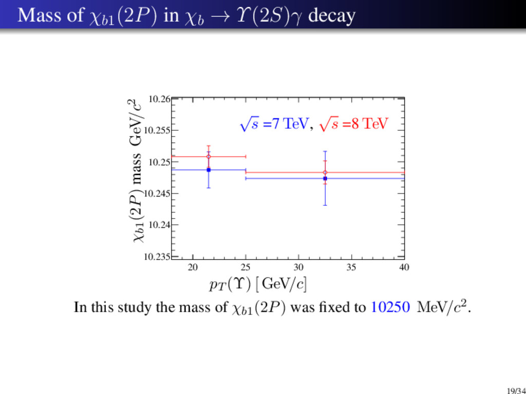
19. Mass of χb1 (2P) in χb → Υ(2S)γ decay 20 25 30 35 40 10.235 10.24 10.245 10.25 10.255 10.26 √ s =7 TeV, √ s =8 TeV χb1(2P) mass GeV/c2 pT (Υ) [ GeV/c] In this study the mass of χb1(2P) was fixed to 10250 MeV/c2. 19/34
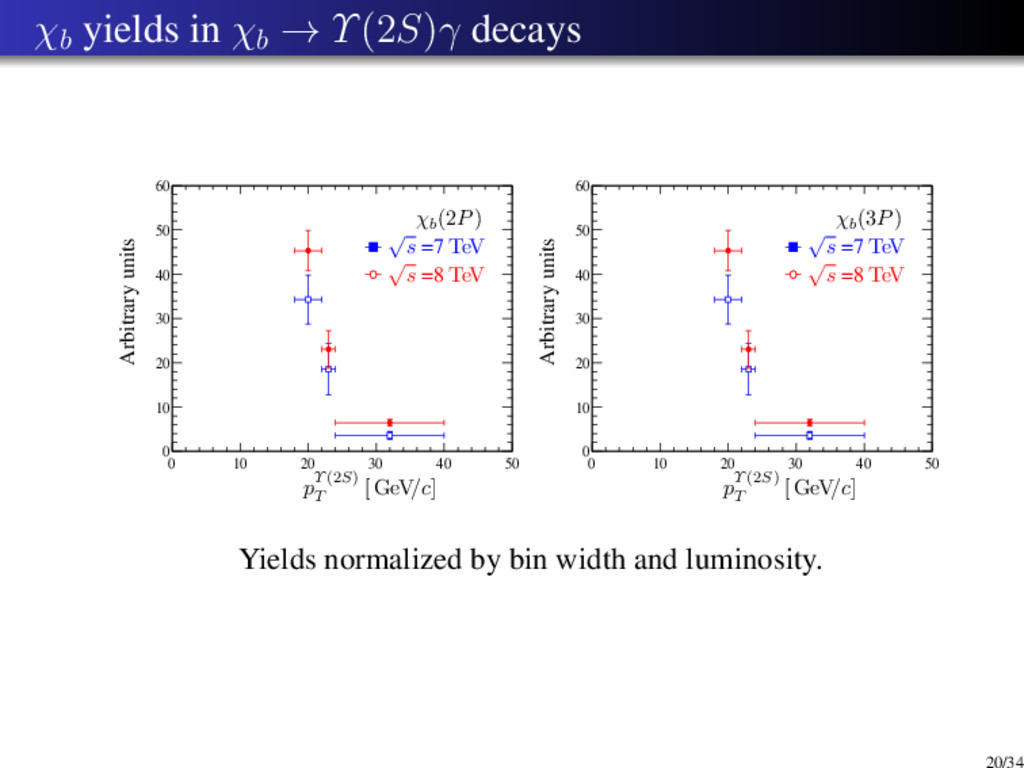
20. χb yields in χb → Υ(2S)γ decays 0 10 20 30 40 50 0 10 20 30 40 50 60 0 10 20 30 40 50 0 10 20 30 40 50 60 Arbitrary units pΥ(2S) T [ GeV/c] χb(2P) Arbitrary units pΥ(2S) T [ GeV/c] χb(3P) √ s =7 TeV √ s =8 TeV √ s =7 TeV √ s =8 TeV Yields normalized by bin width and luminosity. 20/34
21. χb1,2 (3P) → Υ(3S)γ fit model 10.5 10.6 10.7 0 5 10 15 20 25 30 35 40 45 -4 -2 0 2 4 10.5 10.6 10.7 0 2 4 6 8 10 12 14 16 18 -4 -2 0 2 4 Candidates/(20 MeV/c2) m µ+µ−γ − m µ+µ− + 10.3552 GeV/c2 √ s = 8 GeV pT (Υ (3S)) > 27 GeV/c Candidates/(20 MeV/c2) m µ+µ−γ − m µ+µ− + 10.3552 GeV/c2 √ s = 7 GeV pT (Υ (3S)) > 27 GeV/c 2 Crystal Ball for each of χb1,2(3P) signal. Linear combination of basic Bernstein polynomials for combinatorial background. 21/34
22. χb1,2 (3P) → Υ(3S)γ fit model (2) Free parameters: µχb1(3P), yields and background parameters. Linked parameters for χb1 and χb2 signals: µχb2(3P ) = µχb1(3P ) + ∆mtheory χb2(3P ) Nχb = λNχb1 + (1 − λ)Nχb2 σχb2 = σχb1 Fixed parameters from MC study: σχb1(3P ) α and n parameters of CB. Υ(3S) transverse momentum intervals, GeV/c 27 – 40 √ s = 7 TeV √ s = 8 TeV Nχb(3P) 31 ± 12 72 ± 16 Background 97 ± 14 283 ± 21 µχb1(3P) , MeV/c2 10,517 ± 4 10,504.0 ± 2.5 σχb1(3P) , MeV/c2 9 ± 6 8.3 ± 2.7 c0 0.52 ± 0.18 0.52 ± 0.09 c1 -0.42 ± 0.19 -0.36 ± 0.10 c2 1.3 ± 0.8 -1.23 ± 0.18 χ2/n.d.f 0.38 1.09 In this study the mass of χb1(3P) was fixed to the value obtained from the fit performed on both datasets = 10507±2 MeV/c2 22/34
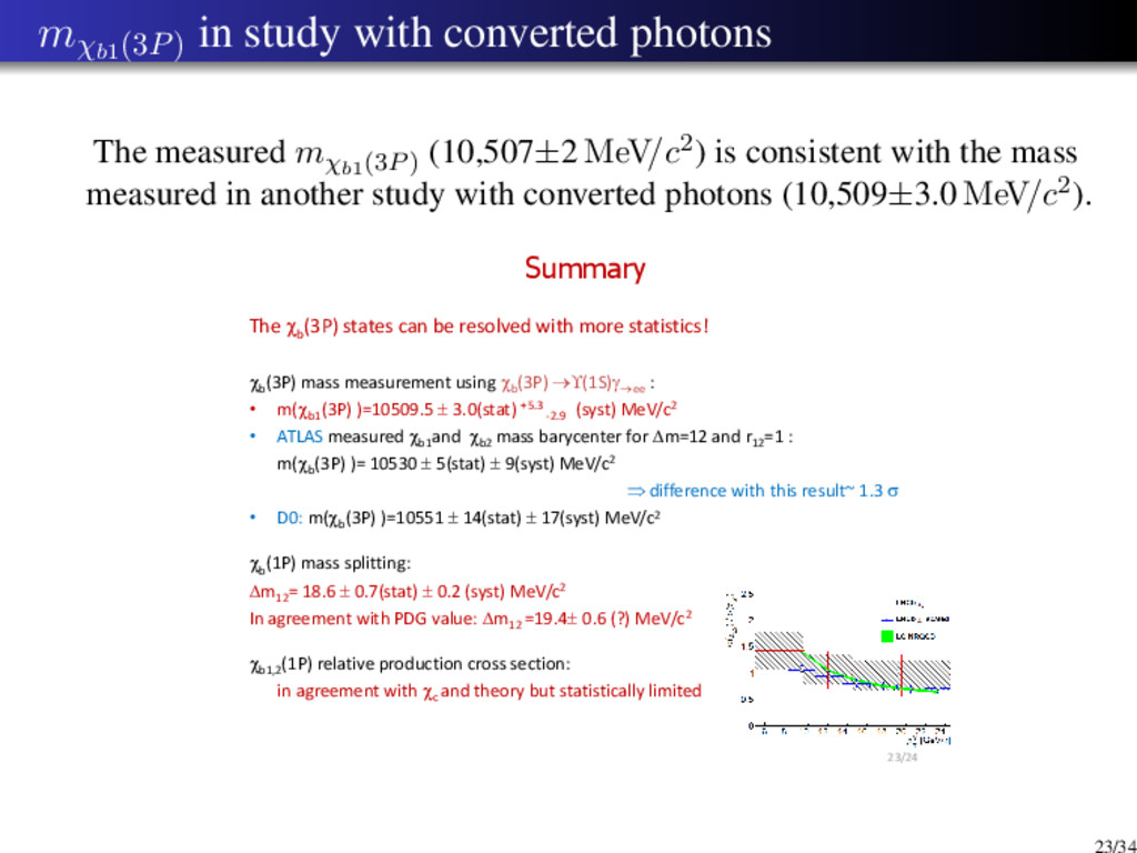
23. mχb1 (3P) in study with converted photons The measured mχb1(3P) (10,507±2 MeV/c2) is consistent with the mass measured in another study with converted photons (10,509±3.0 MeV/c2). Summary The b (3P) states can be resolved with more statistics! b (3P) mass measurement using b (3P) (1S)ee : • m(b1 (3P) )=10509.5  3.0(stat) +5.3 -2.9 (syst) MeV/c2 • ATLAS measured b1 and b2 mass barycenter for m=12 and r12 =1 : m(b (3P) )= 10530  5(stat)  9(syst) MeV/c2  difference with this result~ 1.3  • D0: m(b (3P) )=10551  14(stat)  17(syst) MeV/c2 b (1P) mass splitting: m12 = 18.6  0.7(stat)  0.2 (syst) MeV/c2 In agreement with PDG value: m12 =19.4 0.6 (?) MeV/c2 b1,2 (1P) relative production cross section: in agreement with c and theory but statistically limited 23/24 23/34
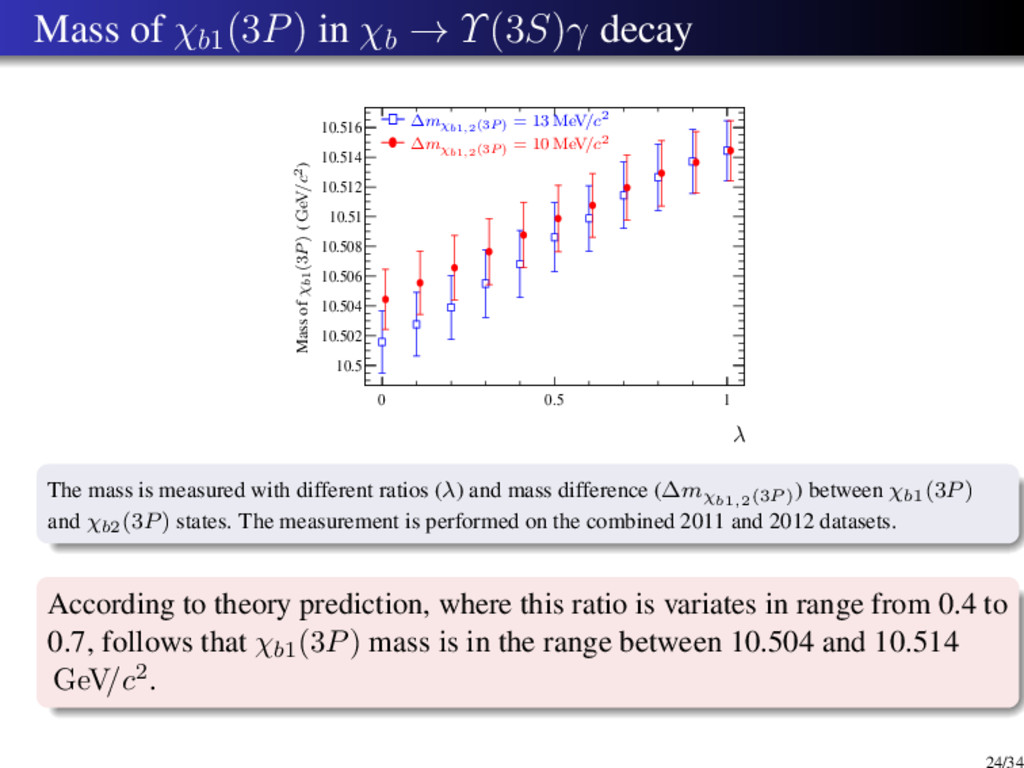
24. Mass of χb1 (3P) in χb → Υ(3S)γ decay 0 0.5 1 10.5 10.502 10.504 10.506 10.508 10.51 10.512 10.514 10.516 Mass of χb1(3P) ( GeV/c2) λ ∆mχb1,2(3P ) = 13 MeV/c2 ∆mχb1,2(3P ) = 10 MeV/c2 The mass is measured with different ratios (λ) and mass difference (∆mχb1,2(3P )) between χb1(3P) and χb2(3P) states. The measurement is performed on the combined 2011 and 2012 datasets. According to theory prediction, where this ratio is variates in range from 0.4 to 0.7, follows that χb1(3P) mass is in the range between 10.504 and 10.514 GeV/c2. 24/34
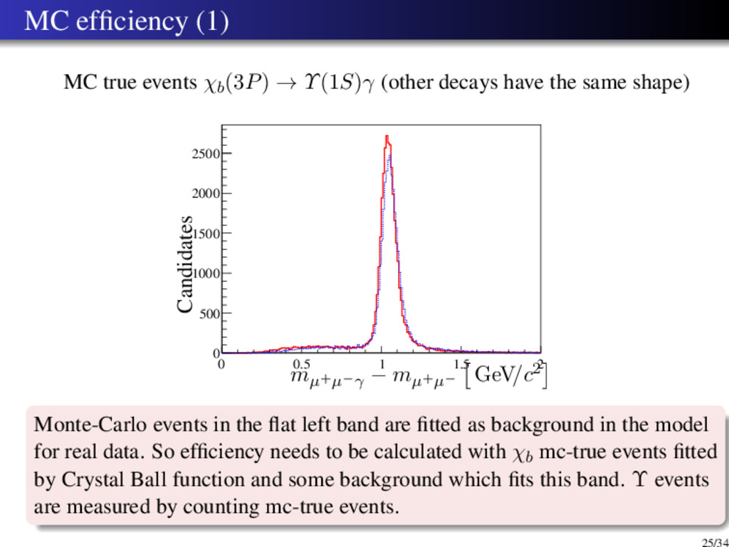
25. MC efficiency (1) MC true events χb(3P) → Υ(1S)γ (other decays have the same shape) 0 0.5 1 1.5 2 0 500 1000 1500 2000 2500 Candidates mµ+µ−γ − mµ+µ− GeV/c2 Monte-Carlo events in the flat left band are fitted as background in the model for real data. So efficiency needs to be calculated with χb mc-true events fitted by Crystal Ball function and some background which fits this band. Υ events are measured by counting mc-true events. 25/34
26. Monte-Carlo photon reconstruction (2) Example of fits: 9.8 9.9 10 10.1 0 1000 2000 3000 4000 5000 6000 -4 -2 0 2 4 χb1(1P) → Υ(1S)γ 6 < pΥ (1S) T < 40 GeV/c mµ+µ−γ − mµ+µ− + 9.4603 GeV/c2 Candidates/(10 MeV/c2) N = 34,330 ± 220 B = 5240 ± 140 (13.3 ± 0.4%) 10 10.2 10.4 10.6 0 500 1000 1500 2000 2500 -4 -2 0 2 4 χb1(2P) → Υ(1S)γ 6 < pΥ (1S) T < 40 GeV/c mµ+µ−γ − mµ+µ− + 9.4603 GeV/c2 Candidates/(10 MeV/c2) N = 22,210 ± 170 B = 2290 ± 90 (9.3 ± 0.4%) 10.2 10.4 10.6 10.8 0 200 400 600 800 1000 1200 1400 -4 -2 0 2 4 χb1(3P) → Υ(1S)γ 6 < pΥ (1S) T < 40 GeV/c mµ+µ−γ − mµ+µ− + 9.4603 GeV/c2 Candidates/(10 MeV/c2) N = 15,110 ± 130 B = 1360 ± 60 (8.26 ± 0.35%) 10.2 10.25 10.3 0 10 20 30 40 50 -4 -2 0 2 4 χb1(2P) → Υ(2S)γ 18 < pΥ (1S) T < 40 GeV/c mµ+µ−γ − mµ+µ− + 10.02326 GeV/c2 Candidates/(10 MeV/c2) N = 194 ± 21 B = 15 ± 17 (7 ± 8%) 10.4 10.5 10.6 0 20 40 60 80 100 120 -4 -2 0 2 4 χb1(3P) → Υ(2S)γ 18 < pΥ (1S) T < 40 GeV/c mµ+µ−γ − mµ+µ− + 10.02326 GeV/c2 Candidates/(10 MeV/c2) N = 672 ± 32 B = 57 ± 21 (7.8 ± 2.9%) 10.45 10.5 10.55 10.6 10.65 0 10 20 30 40 50 60 70 80 -4 -2 0 2 4 χb1(3P) → Υ(3S)γ 27 < pΥ (1S) T < 40 GeV/c mµ+µ−γ − mµ+µ− + 10.355 GeV/c2 Candidates/(10 MeV/c2) N = 154 ± 17 B = 113 ± 16 (42 ± 7%) 26/34
27. Monte-Carlo photon reconstruction efficiency χb(1P), χb(2P), χb(3P) reconstruction efficiency in χb → Υγ decays. 10 15 20 25 30 0 5 10 15 20 25 30 35 20 25 30 35 40 0 5 10 15 20 25 30 35 Efficiency (%) pT (Υ(1S)) GeV/c2 χb(1, 2, 3P ) → Υ (1S)γ Efficiency (%) pT (Υ(2S)) GeV/c2 χb(2, 3P ) → Υ (2S)γ Photons is more energetic as pT (Υ) increases so it is reconstructed more efficiently. 27/34
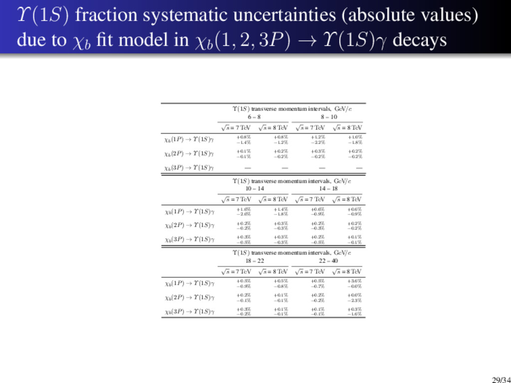
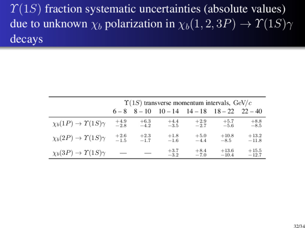
28. Systematic uncertainties Since this analysis measures the fraction of Υ(nS) particles originating from χb decays, most systematic uncertainties cancel in the ratio and only residual effects need to be taken into account. Systematic uncertainties on the event yields are mostly due to the fit model of Υ and χb invariant masses, while the ones on the efficiency are due to the photon reconstruction and the unknown initial polarization of χb and Υ particles. 28/34
29. Υ(1S) fraction systematic uncertainties (absolute values) due to χb fit model in χb (1, 2, 3P) → Υ(1S)γ decays Υ(1S) transverse momentum intervals, GeV/c 6 – 8 8 – 10 √ s = 7 TeV √ s = 8 TeV √ s = 7 TeV √ s = 8 TeV χb(1P) → Υ(1S)γ +0.8% −1.4% +0.8% −1.2% +1.2% −2.2% +1.0% −1.8% χb(2P) → Υ(1S)γ +0.1% −0.1% +0.2% −0.2% +0.3% −0.2% +0.2% −0.2% χb(3P) → Υ(1S)γ — — — — Υ(1S) transverse momentum intervals, GeV/c 10 – 14 14 – 18 √ s = 7 TeV √ s = 8 TeV √ s = 7 TeV √ s = 8 TeV χb(1P) → Υ(1S)γ +1.0% −2.0% +1.4% −1.8% +0.6% −0.9% +0.6% −0.9% χb(2P) → Υ(1S)γ +0.2% −0.2% +0.3% −0.3% +0.2% −0.3% +0.2% −0.2% χb(3P) → Υ(1S)γ +0.3% −0.5% +0.3% −0.3% +0.2% −0.5% +0.1% −0.1% Υ(1S) transverse momentum intervals, GeV/c 18 – 22 22 – 40 √ s = 7 TeV √ s = 8 TeV √ s = 7 TeV √ s = 8 TeV χb(1P) → Υ(1S)γ +0.5% −0.9% +0.5% −0.8% +0.5% −0.7% +3.6% −0.0% χb(2P) → Υ(1S)γ +0.2% −0.1% +0.1% −0.1% +0.2% −0.2% +0.0% −2.3% χb(3P) → Υ(1S)γ +0.3% −0.2% +0.1% −0.1% +0.1% −0.1% +0.3% −1.6% 29/34
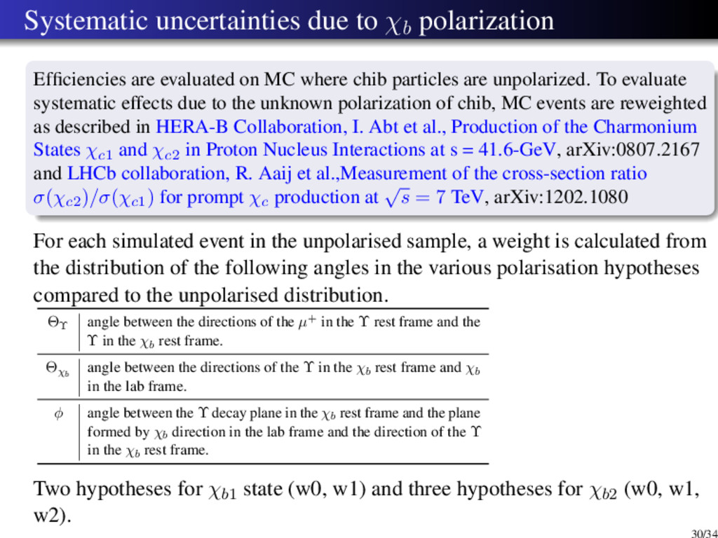
30. Systematic uncertainties due to χb polarization Efficiencies are evaluated on MC where chib particles are unpolarized. To evaluate systematic effects due to the unknown polarization of chib, MC events are reweighted as described in HERA-B Collaboration, I. Abt et al., Production of the Charmonium States χc1 and χc2 in Proton Nucleus Interactions at s = 41.6-GeV, arXiv:0807.2167 and LHCb collaboration, R. Aaij et al.,Measurement of the cross-section ratio σ(χc2 )/σ(χc1 ) for prompt χc production at √ s = 7 TeV, arXiv:1202.1080 For each simulated event in the unpolarised sample, a weight is calculated from the distribution of the following angles in the various polarisation hypotheses compared to the unpolarised distribution. ΘΥ angle between the directions of the µ+ in the Υ rest frame and the Υ in the χb rest frame. Θχb angle between the directions of the Υ in the χb rest frame and χb in the lab frame. φ angle between the Υ decay plane in the χb rest frame and the plane formed by χb direction in the lab frame and the direction of the Υ in the χb rest frame. Two hypotheses for χb1 state (w0, w1) and three hypotheses for χb2 (w0, w1, w2). 30/34
31. Systematic uncertainties due to χb polarization The ratio of efficiency for unpolarized χb to efficiency for polarized χb. (1S) Υ T p 10 20 30 40 w0 γ ε / unpol γ ε 0.92 0.94 0.96 0.98 1 1.02 1.04 1.06 1.08 1.1 γ (1S) Υ → (1P) b2 χ w0, γ (1S) Υ → (1P) b2 χ w0, (1S) Υ T p 10 20 30 40 w1 γ ε / unpol γ ε 0.94 0.96 0.98 1 1.02 1.04 1.06 γ (1S) Υ → (1P) b2 χ w1, γ (1S) Υ → (1P) b2 χ w1, (1S) Υ T p 10 20 30 40 w2 γ ε / unpol γ ε 0.94 0.96 0.98 1 1.02 1.04 1.06 γ (1S) Υ → (1P) b2 χ w2, γ (1S) Υ → (1P) b2 χ w2, The efficiency in the different polarization scenarios is consistent with the unpolarized one. We conservatively take the statistical uncertainty on the efficiency ratio as systematic uncertainty due to the χb polarization. 31/34
32. Υ(1S) fraction systematic uncertainties (absolute values) due to unknown χb polarization in χb (1, 2, 3P) → Υ(1S)γ decays Υ(1S) transverse momentum intervals, GeV/c 6 – 8 8 – 10 10 – 14 14 – 18 18 – 22 22 – 40 χb(1P) → Υ(1S)γ +4.9 −2.8 +6.3 −4.2 +4.4 −3.5 +2.9 −2.7 +5.7 −5.6 +8.8 −8.5 χb(2P) → Υ(1S)γ +2.6 −1.5 +2.3 −1.7 +1.8 −1.6 +5.0 −4.4 +10.8 −8.5 +13.2 −11.8 χb(3P) → Υ(1S)γ — — +3.7 −3.2 +8.4 −7.0 +13.6 −10.4 +15.5 −12.7 32/34
33. Υ fractions in χb → Υγ decays 10 20 30 40 0 5 10 15 20 25 30 35 40 45 50 Υ(1S) fraction, % pΥ(1S) T [ GeV/c] χb(1P) → Υ(1S)γ √ s =7 TeV √ s =8 TeV 10 20 30 40 0 5 10 15 20 25 30 35 40 45 50 Υ(1S) fraction, % pΥ(1S) T [ GeV/c] χb(2P) → Υ(1S)γ √ s =7 TeV √ s =8 TeV 10 20 30 40 0 5 10 15 20 25 30 35 40 45 50 Υ(1S) fraction, % pΥ(1S) T [ GeV/c] χb(3P) → Υ(1S)γ √ s =7 TeV √ s =8 TeV 10 20 30 40 0 5 10 15 20 25 30 35 40 45 50 Υ(2S) fraction, % pΥ(2S) T [ GeV/c] χb(2P) → Υ(2S)γ √ s =7 TeV √ s =8 TeV 10 20 30 40 0 5 10 15 20 25 30 35 40 45 50 Υ(2S) fraction, % pΥ(2S) T [ GeV/c] χb(3P) → Υ(2S)γ √ s =7 TeV √ s =8 TeV 10 20 30 40 0 10 20 30 40 50 60 70 80 90 100 Υ(3S) fraction, % pΥ(3S) T [ GeV/c] χb(3P) → Υ(3S)γ √ s =7 TeV √ s =8 TeV 10 20 30 40 0 5 10 15 20 25 30 35 40 45 50 Υ(1S) fraction, % pΥ(1S) T [ GeV/c] χb(1P) → Υ(1S)γ √ s =7 TeV √ s =8 TeV √ s =7 TeV (2010) Outer error bars show statistical and systematics errors, inner error bars — only statistical errors. 33/34
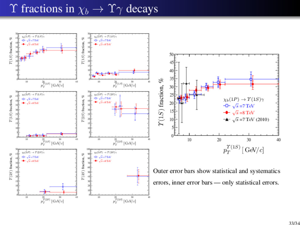
34. Summary Measured fractions of Υ(1, 2, 3S) originated from χb decays. About 40% of Υ come from χb, with mild dependence on Υ transverse momentum. Estimated the mass χb(3P) mass: between 10,504 and 10,512 MeV/c2; consistent with another determination which uses converted photons. LHCb analysis note: https://twiki.cern.ch/twiki/bin/viewauth/LHCbPhysics/ChiB2fb 34/34