A note on the characterization of optimal allocations in OLG models with multiple goods

by L. Rakotonindrainy

Transcript

1. Introduction The model Characterization of Pareto optimal allocations Sketch of the proof Notes on the Characterization of optimal allocations in OLG models wilth multiple goods Lalaina Rakotonindrainy (joint work with Jean-Marc Bonnisseau) Universit´ e de Paris 1 Panth´ eon–Sorbone, Paris School of Economics Journ´ ees du GdR MOA 2–4 December 2015
2. Introduction The model Characterization of Pareto optimal allocations Sketch of the proof A canonical OLG model • Infinitely many dates (t = 1, 2 · · · ) • At each date t, there exists a finite set Lt of commodities available in the market. • At each period t ∈ N, a finite and non-empty set of consumers It is born, called generation t. Each individual lives within two periods: young at date t then old at t + 1. • each consumer i of each generation t is characterized by her consumption set Xi = RLt + × R Lt+1 + , a preference Pi over Xi (or a utility function ui ), a strictly positive initial endowment ei = (ei t , ei t+1 ), during her two-periods lifetime. • Market failure in OLG models: equilibria may lack in being Pareto optimal
3. Introduction The model Characterization of Pareto optimal allocations Sketch of the proof Notations: ¯ et = i∈It−1∪It ei t Definition x feasible is Pareto optimal (PO) (resp. weakly Pareto optimal (WPO)) if there is no (yi ) in i∈I Xi such that: i∈It−1∪It yi t = ¯ et, for t ≥ 1 and for all i ∈ I, yi ∈ ¯ Pi (xi ), with yi ∈ Pi (xi ) for at least one individual i (resp. ∃¯ t such that ∀t ≥ ¯ t, ∀i ∈ It yi = xi ).
4. Introduction The model Characterization of Pareto optimal allocations Sketch of the proof • Every Walrasian allocation is WPO, and every WPO allocation is supported by a price sequence and is a Walrasian allocation. Thus from WPO to PO: a characterization is needed. • Balasko & Shell’s characterization (1980): use curvature concept of indifference surfaces to strengthen strict concavity of utility functions, proof relies on the special case of one commodity then extension to multiple commodities is sketched
5. Introduction The model Characterization of Pareto optimal allocations Sketch of the proof Purpose • provide a simpler, direct proof of the Balasko-Shell Criterion considering in one step several consumers for each generation and several commodities • encompass the case of non-complete, non-transitive preferences • compute explicitly a Pareto improving transfer when the allocation does not satisfy the Balasko-Shell Criterion • Approach: More geometric and set-theoretic: assumptions on the (weakly) preferred sets and the associated normal cones • But proof strongly based on Balasko & Shell’s one!
6. Introduction The model Characterization of Pareto optimal allocations Sketch of the proof A standard OLG exchange economy E • for each consumer i, a strict preference relation Pi from Xi to Xi • weakly preferred set ¯ Pi (xi ): zi ∈ ¯ Pi (xi ) if and only if zi is preferred or indifferent to xi . • N¯ Pi (xi ) (xi ) = {q ∈ RL × RL | q · (z − xi ) ≤ 0, ∀z ∈ ¯ Pi (xi )} Assumption A. • a) For all i in I, Pi (xi ) open in X, convex, xi ∈ ¯ Pi (xi ) and xi / ∈ Pi (xi ), Pi (xi ) + (RLt + × R Lt+1 + ) ⊂ Pi (xi ). • b) For all i ∈ I, for all xi in the interior of Xi , −N¯ Pi (xi ) (xi ) is a half line {µγi (xi ) | µ ≥ 0}, γi (xi ) ∈ RLt ++ × R Lt+1 ++ continuous mapping on the interior of Xi , γi (xi ) = 1.
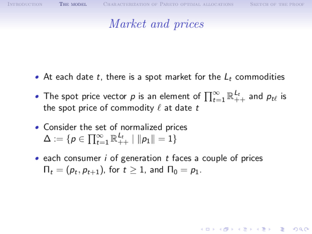
7. Introduction The model Characterization of Pareto optimal allocations Sketch of the proof Market and prices • At each date t, there is a spot market for the Lt commodities • The spot price vector p is an element of ∞ t=1 RLt ++ and pt is the spot price of commodity at date t • Consider the set of normalized prices ∆ := {p ∈ ∞ t=1 RLt ++ | p1 = 1} • each consumer i of generation t faces a couple of prices Πt = (pt, pt+1), for t ≥ 1, and Π0 = p1.
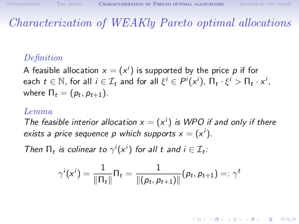
8. Introduction The model Characterization of Pareto optimal allocations Sketch of the proof Characterization of WEAKly Pareto optimal allocations Definition A feasible allocation x = (xi ) is supported by the price p if for each t ∈ N, for all i ∈ It and for all ξi ∈ Pi (xi ), Πt · ξi > Πt · xi , where Πt = (pt, pt+1). Lemma The feasible interior allocation x = (xi ) is WPO if and only if there exists a price sequence p which supports x = (xi ). Then Πt is colinear to γi (xi ) for all t and i ∈ It: γi (xi ) = 1 Πt Πt = 1 (pt, pt+1) (pt, pt+1) =: γt
9. Introduction The model Characterization of Pareto optimal allocations Sketch of the proof Additional assumptions Let x = (xi ) ∈ i∈I Xi a WPO allocation, such that:
10. Introduction The model Characterization of Pareto optimal allocations Sketch of the proof Additional assumptions Let x = (xi ) ∈ i∈I Xi a WPO allocation, such that: • Assumption B: there exist ¯ χ > 0 and χ > 0 such that for all t ≥ 1, ¯ et ≤ ¯ χ1Lt , for all t ≥ 1, χ(1Lt , 1Lt+1 ) ≤ xi for all i ∈ It and χ1L1 ≤ xi for all i ∈ I0;
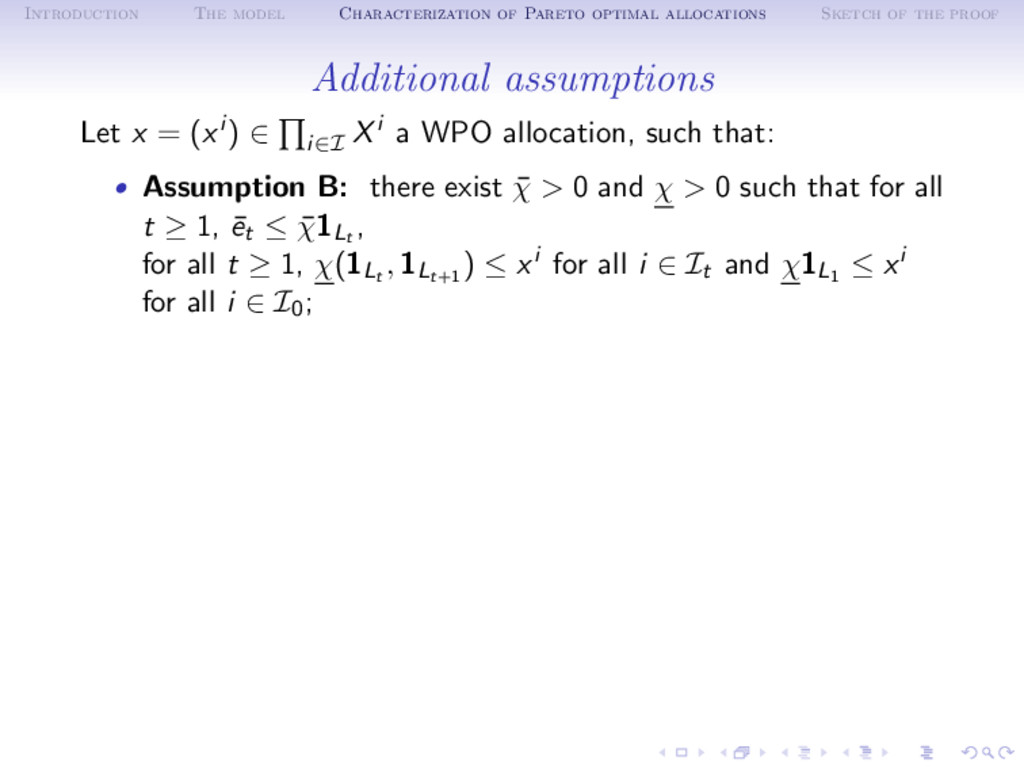
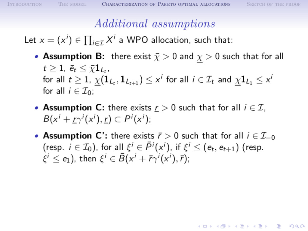
11. Introduction The model Characterization of Pareto optimal allocations Sketch of the proof Additional assumptions Let x = (xi ) ∈ i∈I Xi a WPO allocation, such that: • Assumption B: there exist ¯ χ > 0 and χ > 0 such that for all t ≥ 1, ¯ et ≤ ¯ χ1Lt , for all t ≥ 1, χ(1Lt , 1Lt+1 ) ≤ xi for all i ∈ It and χ1L1 ≤ xi for all i ∈ I0; • Assumption C: there exists r > 0 such that for all i ∈ I, B(xi + rγi (xi ), r) ⊂ Pi (xi ); • Assumption C’: there exists ¯ r > 0 such that for all i ∈ I−0 (resp. i ∈ I0), for all ξi ∈ ¯ Pi (xi ), if ξi ≤ (et, et+1) (resp. ξi ≤ e1), then ξi ∈ ¯ B(xi + ¯ rγi (xi ), ¯ r);
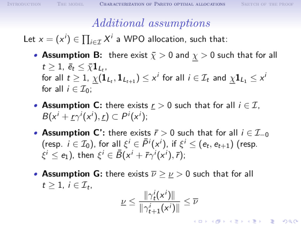
12. Introduction The model Characterization of Pareto optimal allocations Sketch of the proof Additional assumptions Let x = (xi ) ∈ i∈I Xi a WPO allocation, such that: • Assumption B: there exist ¯ χ > 0 and χ > 0 such that for all t ≥ 1, ¯ et ≤ ¯ χ1Lt , for all t ≥ 1, χ(1Lt , 1Lt+1 ) ≤ xi for all i ∈ It and χ1L1 ≤ xi for all i ∈ I0; • Assumption C: there exists r > 0 such that for all i ∈ I, B(xi + rγi (xi ), r) ⊂ Pi (xi ); • Assumption C’: there exists ¯ r > 0 such that for all i ∈ I−0 (resp. i ∈ I0), for all ξi ∈ ¯ Pi (xi ), if ξi ≤ (et, et+1) (resp. ξi ≤ e1), then ξi ∈ ¯ B(xi + ¯ rγi (xi ), ¯ r); • Assumption G: there exists ν ≥ ν > 0 such that for all t ≥ 1, i ∈ It, ν ≤ γi t (xi ) γi t+1 (xi ) ≤ ν
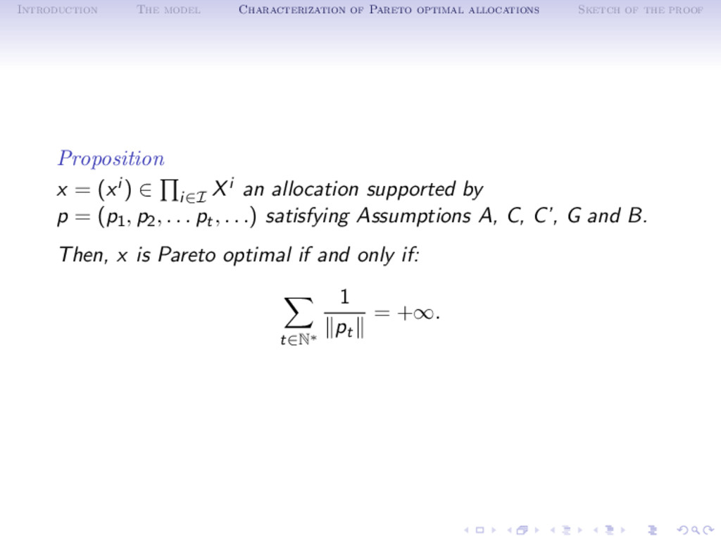
13. Introduction The model Characterization of Pareto optimal allocations Sketch of the proof Proposition x = (xi ) ∈ i∈I Xi an allocation supported by p = (p1, p2, . . . pt, . . .) satisfying Assumptions A, C, C’, G and B. Then, x is Pareto optimal if and only if: t∈N∗ 1 pt = +∞.
14. Introduction The model Characterization of Pareto optimal allocations Sketch of the proof • Assumption B implies that the number of individuals is uniformly bounded above at each generation by some ¯ I. • Assumptions C and C’ still hold when we aggregate the finitely many consumers i ∈ It at each period t. • Since the allocation x = (xi ) is PO iff there is no feasible aggregate Pareto improving transfer upon x ⇒ construct and characterize a sequence of aggregate Pareto improving transfers.
15. Introduction The model Characterization of Pareto optimal allocations Sketch of the proof Aggregation: one consumer at each generation ¯ Pt((xi )) := i∈It ¯ Pi (xi ) ¯ xt := i∈It xi N¯ Pt ((xi )) (¯ xt) = i∈It N¯ Pi (xi ) (xi ) = {λΠt | λ ≥ 0} = {λγt | λ ≥ 0} • x = (xi ) PO iff ¯ x Pareto optimal for the preference relation ¯ Pt, i.e no feasible aggregate Pareto improving transfer. • If x supported by a price, then ¯ x supported by the same price.
16. Introduction The model Characterization of Pareto optimal allocations Sketch of the proof A geometric approach • Feasible aggregate transfer: ¯ h = (¯ ht t , ¯ ht t+1 ) with ¯ ht t+1 = −¯ ht+1 t+1 . • Net present value: ηt = Πt · ¯ ht • αt = ¯ ht 2 Πt ηt • ¯ ht ≤ αt: α bounded ⇒ ¯ h bounded. • αt 2 actually represents the radius of the sphere S(xt + αt 2 γt, αt 2 ) which is tangent to ¯ Pt((xi )) at xt, and contains xt + ¯ ht: xt + ¯ ht − xt + αt 2 γt = αt 2
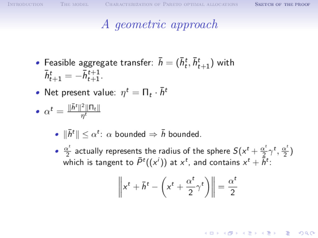
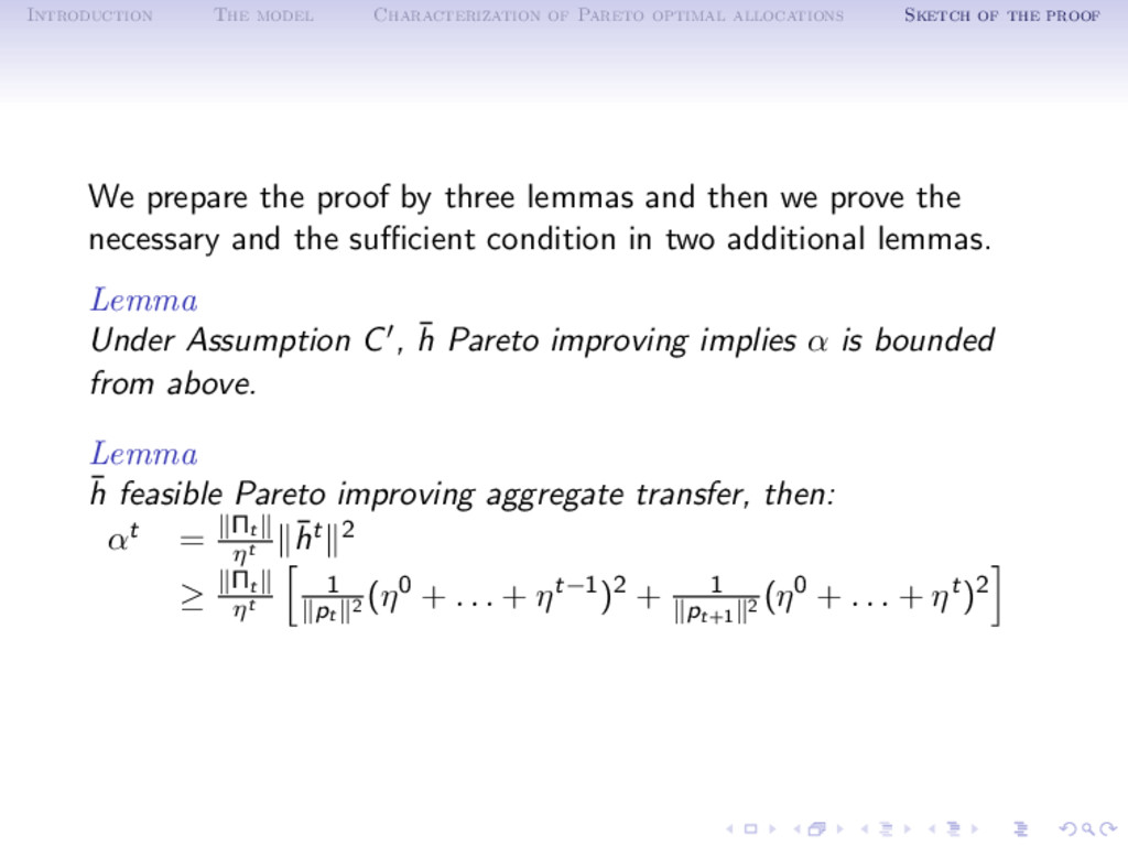
17. Introduction The model Characterization of Pareto optimal allocations Sketch of the proof We prepare the proof by three lemmas and then we prove the necessary and the sufficient condition in two additional lemmas. Lemma Under Assumption C , ¯ h Pareto improving implies α is bounded from above. Lemma ¯ h feasible Pareto improving aggregate transfer, then: αt = Πt ηt ¯ ht 2 ≥ Πt ηt 1 pt 2 (η0 + . . . + ηt−1)2 + 1 pt+1 2 (η0 + . . . + ηt)2
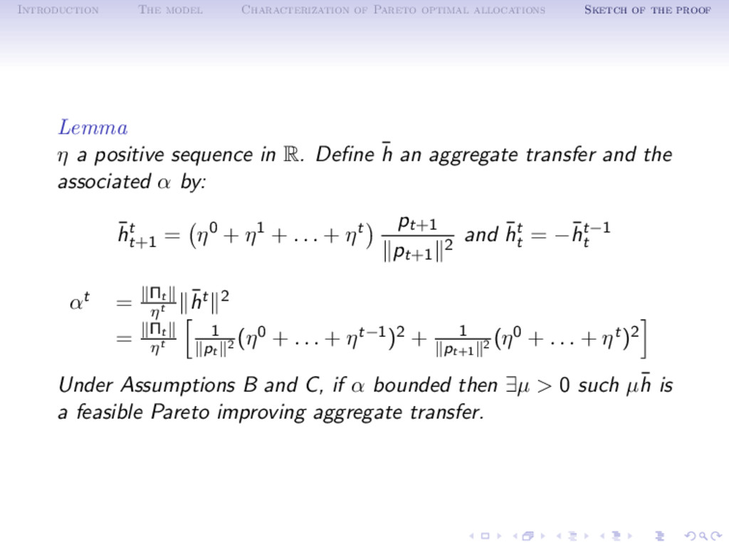
18. Introduction The model Characterization of Pareto optimal allocations Sketch of the proof Lemma η a positive sequence in R. Define ¯ h an aggregate transfer and the associated α by: ¯ ht t+1 = η0 + η1 + . . . + ηt pt+1 pt+1 2 and ¯ ht t = −¯ ht−1 t αt = Πt ηt ¯ ht 2 = Πt ηt 1 pt 2 (η0 + . . . + ηt−1)2 + 1 pt+1 2 (η0 + . . . + ηt)2 Under Assumptions B and C, if α bounded then ∃µ > 0 such µ¯ h is a feasible Pareto improving aggregate transfer.
19. Introduction The model Characterization of Pareto optimal allocations Sketch of the proof Lemma Given the positive price sequence p, if x is not PO, then under Assumption C , t∈N∗ 1 pt < +∞.
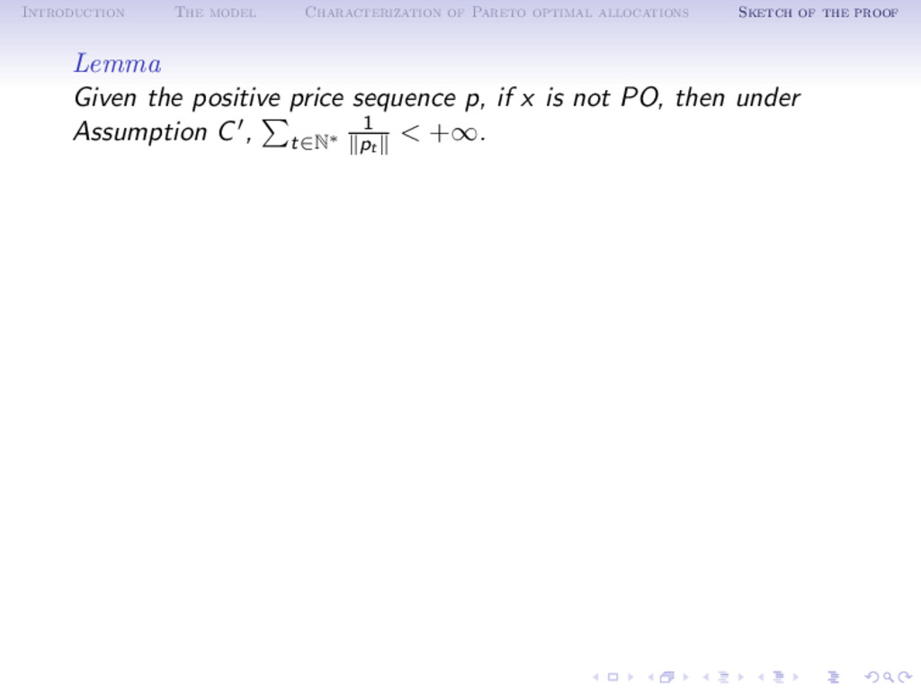
20. Introduction The model Characterization of Pareto optimal allocations Sketch of the proof Lemma Given the positive price sequence p, if x is not PO, then under Assumption C , t∈N∗ 1 pt < +∞. • one commodity and one consumer per generation, • P((1, 1)) = {ξ ∈ R2 + | tξ1 + (t + 1)ξt+1 > 2t + 1} • (1, 1) is supported by the price (1, 2, . . . , t, . . .) and t 1 pt = t 1 t = +∞, • but (1 2 , 3 2 ) for each generation P-dominates (1, 1)
21. Introduction The model Characterization of Pareto optimal allocations Sketch of the proof Lemma Under Assumptions B, C and G, if the positive price sequence p satisfies t 1 pt < +∞, then x is not PO.
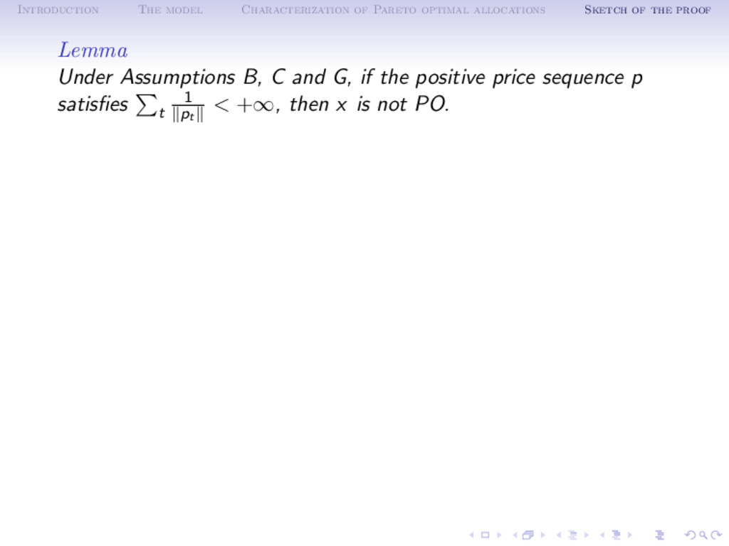
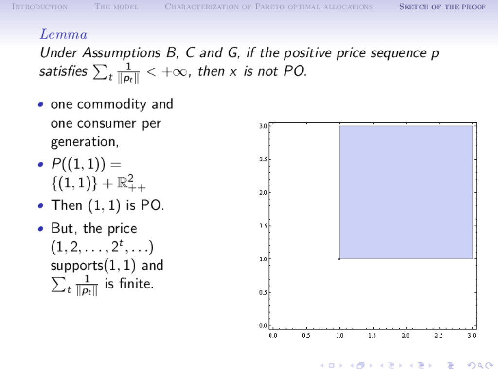
22. Introduction The model Characterization of Pareto optimal allocations Sketch of the proof Lemma Under Assumptions B, C and G, if the positive price sequence p satisfies t 1 pt < +∞, then x is not PO. • one commodity and one consumer per generation, • P((1, 1)) = {(1, 1)} + R2 ++ • Then (1, 1) is PO. • But, the price (1, 2, . . . , 2t, . . .) supports(1, 1) and t 1 pt is finite.
23. Conclusion • Result relies on the fact that proof is direct, simpler in the sense that it allows to directly tackle the multi commodities case and gives explicit form of Pareto improving transfers when not PO • Optimality characterization to the non conventional case where the consumptions sets are not the positive orthant, as in the OLG with durable goods. • Extension to the more general case of heterogeneous lifetimes within each generation
24. Thank you for your attention.
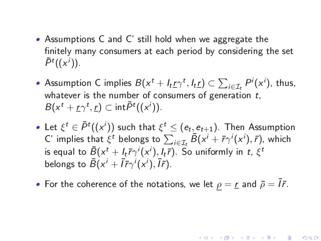
25. • Assumptions C and C’ still hold when we aggregate the finitely many consumers at each period by considering the set ¯ Pt((xi )). • Assumption C implies B(xt + Itrγt, Itr) ⊂ i∈It Pi (xi ), thus, whatever is the number of consumers of generation t, B(xt + rγt, r) ⊂ int ¯ Pt((xi )). • Let ξt ∈ ¯ Pt((xi )) such that ξt ≤ (et, et+1). Then Assumption C’ implies that ξt belongs to i∈It ¯ B(xi + ¯ rγi (xi ), ¯ r), which is equal to ¯ B(xt + It ¯ rγi (xi ), It ¯ r). So uniformly in t, ξt belongs to ¯ B(xi + ¯ I ¯ rγi (xi ), ¯ I ¯ r). • For the coherence of the notations, we let ρ = r and ¯ ρ = ¯ I ¯ r.
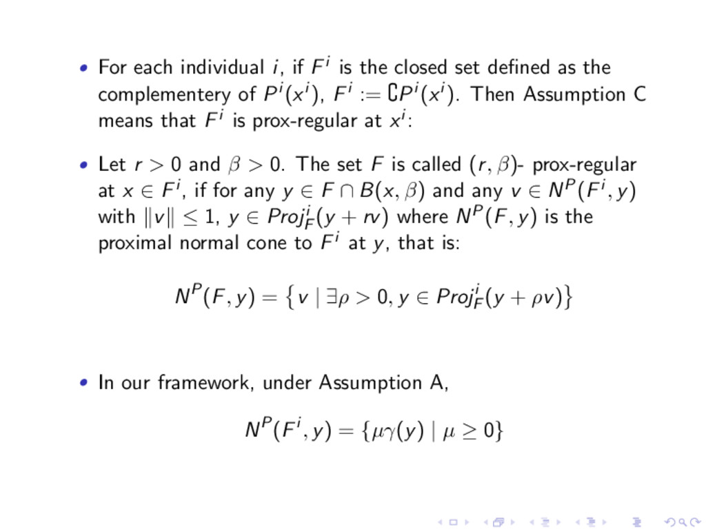
26. • For each individual i, if Fi is the closed set defined as the complementery of Pi (xi ), Fi := Pi (xi ). Then Assumption C means that Fi is prox-regular at xi : • Let r > 0 and β > 0. The set F is called (r, β)- prox-regular at x ∈ Fi , if for any y ∈ F ∩ B(x, β) and any v ∈ NP(Fi , y) with v ≤ 1, y ∈ Proji F (y + rv) where NP(F, y) is the proximal normal cone to Fi at y, that is: NP(F, y) = v | ∃ρ > 0, y ∈ Proji F (y + ρv) • In our framework, under Assumption A, NP(Fi , y) = {µγ(y) | µ ≥ 0}