PTQ: Post-Training Quantization

東京大学理学部情報科学科（通称理情）には、情報科学演習Ⅲ（通称演習3）という授業が存在し、そこでは計3つの研究室を訪問した上で、それぞれの研究室で短期間のプロジェクトに取り組みます。このスライドは、私が高前田研究室を訪問したときに、post-training quantization (PTQ)について調査したものです。

This slides explain post-training quantization (PTQ).

Transcript

1. Handy but powerful quantization of DNNs Masayuki Usui April 18, 2022
2. Agenda Explain the basics of quantization Present recent techniques that alleviate the performance drop due to quantization Show the effect of these techniques citing the experimental results from the literature
3. Contents Basics Quantization range setting Equalization Absorbing bias Bias correction AdaRound References
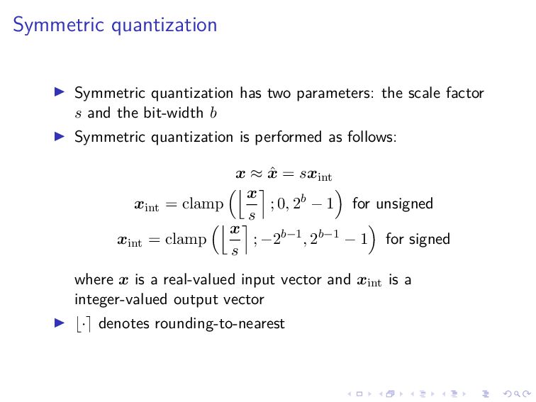
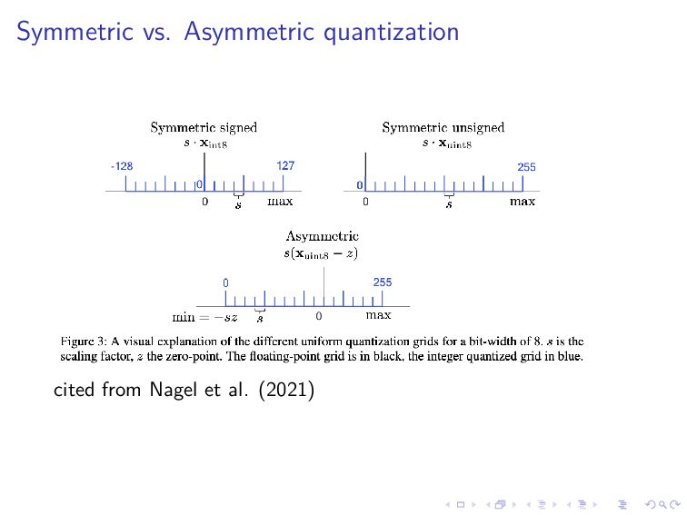
4. Symmetric quantization Symmetric quantization has two parameters: the scale factor s and the bit-width b Symmetric quantization is performed as follows: x ≈ ˆ x = sxint xint = clamp x s ; 0, 2b − 1 for unsigned xint = clamp x s ; −2b−1, 2b−1 − 1 for signed where x is a real-valued input vector and xint is a integer-valued output vector · denotes rounding-to-nearest
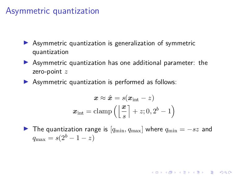
5. Asymmetric quantization Asymmetric quantization is generalization of symmetric quantization Asymmetric quantization has one additional parameter: the zero-point z Asymmetric quantization is performed as follows: x ≈ ˆ x = s(xint − z) xint = clamp x s + z; 0, 2b − 1 The quantization range is [qmin, qmax] where qmin = −sz and qmax = s(2b − 1 − z)
6. Symmetric vs. Asymmetric quantization cited from Nagel et al. (2021)
7. Quantization granularity Per-tensor quantization: a quantizer (i.e. a quantization parameter) per tensor Per-channel quantization: a quantizer per output channel (for weight tensors) Further granularity is actively explored in many papers
8. Quantization range setting There are several ways to determine quantization ranges In the Min-Max method qmin = min i,j Vi,j qmax = max i,j Vi,j where V is a tensor In the MSE based approach argmin qmin,qmax V − ˆ V 2 F where V is a tensor, ˆ V is the quantized version of V , and · F is the Frobenius norm
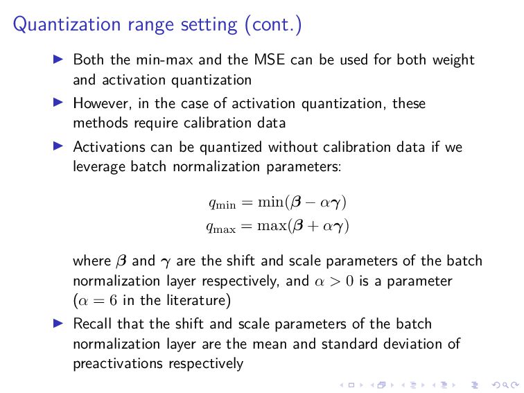
9. Quantization range setting (cont.) Both the min-max and the MSE can be used for both weight and activation quantization However, in the case of activation quantization, these methods require calibration data Activations can be quantized without calibration data if we leverage batch normalization parameters: qmin = min(β − αγ) qmax = max(β + αγ) where β and γ are the shift and scale parameters of the batch normalization layer respectively, and α > 0 is a parameter (α = 6 in the literature) Recall that the shift and scale parameters of the batch normalization layer are the mean and standard deviation of preactivations respectively
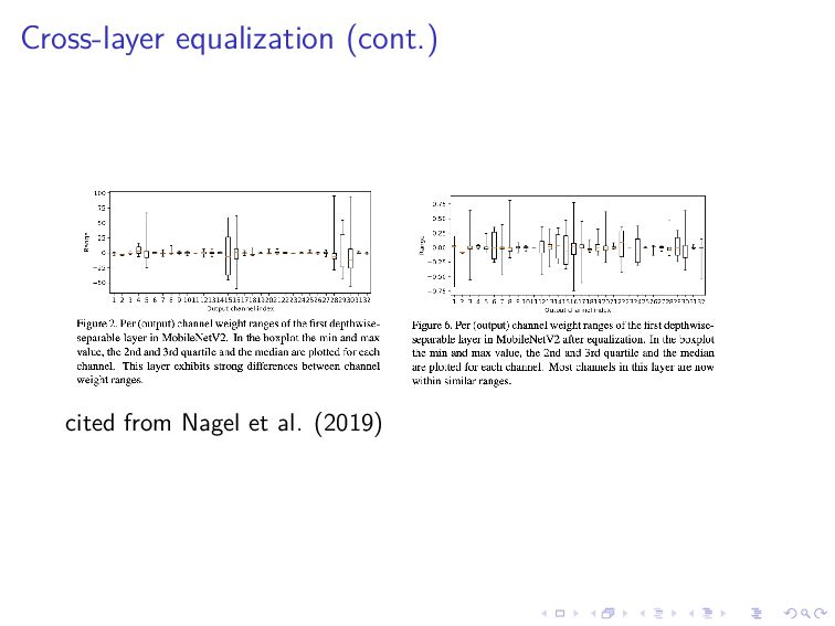
10. Cross-layer equalization If the weight distribution vary greatly from channel to channel, per-tensor quantization might not work well This actually happens in depthwise separable convolution layers The solution is to scale weight tensors
11. Cross-layer equalization (cont.) The key is the positive scaling property that some activation functions have: f(sx) = sf(x) where f is a activation function and s is a positive real number The ReLU has this property since ReLU(sx) = sReLU(x) holds for any positive real number s and any real number x
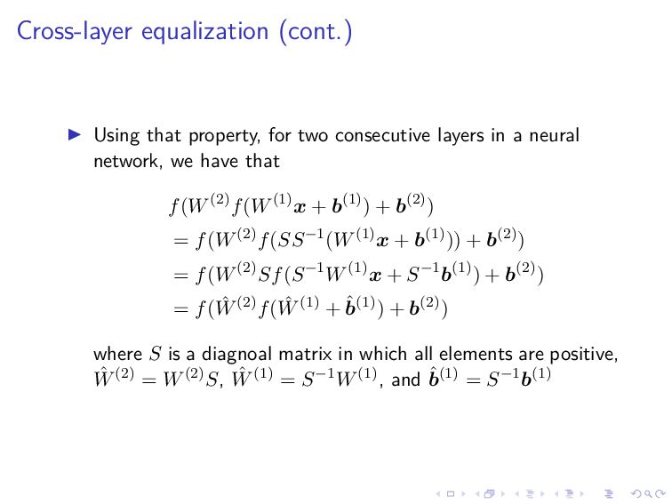
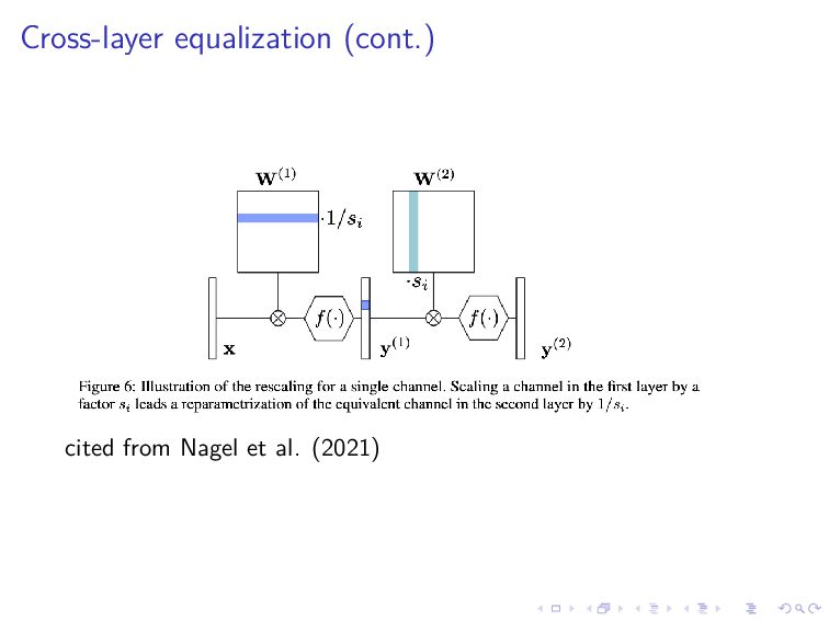
12. Cross-layer equalization (cont.) Using that property, for two consecutive layers in a neural network, we have that f(W(2)f(W(1)x + b(1)) + b(2)) = f(W(2)f(SS−1(W(1)x + b(1))) + b(2)) = f(W(2)Sf(S−1W(1)x + S−1b(1)) + b(2)) = f( ˆ W(2)f( ˆ W(1) + ˆ b(1)) + b(2)) where S is a diagnoal matrix in which all elements are positive, ˆ W(2) = W(2)S, ˆ W(1) = S−1W(1), and ˆ b(1) = S−1b(1)
13. Cross-layer equalization (cont.) cited from Nagel et al. (2021)
14. Cross-layer equalization (cont.) We want to find S that makes the ranges of each channel similar so that the quantization error would be small Formally, we maximize i p(1) i p(2) i where p(k) i is the precision of channel i in ˆ W(k) Formally, p(k) i is defined by p(k) i = ˆ r(k) i ˆ R(k) where ˆ r(k) i is the range of channel i in ˆ W(k) and ˆ R(k) is the total range of ˆ W(k)
15. Cross-layer equalization (cont.) Note that ˆ r(1) i = 2 max j | ˆ W(1) ij | ˆ r(2) i = 2 max j | ˆ W(2) ji | holds for symmetric quantization In the case of symmetric quantization, the solution of the optimization problem is shown to be si = 1 r(2) i r(1) i r(2) i where S = diag(s1, . . . , sn) This solution leads to ˆ r(1) i = ˆ r(2) i = r(1) i r(2) i for all i
16. Cross-layer equalization (cont.) cited from Nagel et al. (2019)
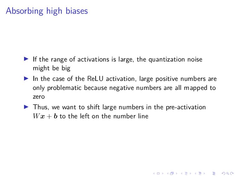
17. Absorbing high biases If the range of activations is large, the quantization noise might be big In the case of the ReLU activation, large positive numbers are only problematic because negative numbers are all mapped to zero Thus, we want to shift large numbers in the pre-activation Wx + b to the left on the number line
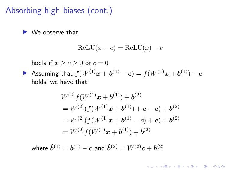
18. Absorbing high biases (cont.) We observe that ReLU(x − c) = ReLU(x) − c hodls if x ≥ c ≥ 0 or c = 0 Assuming that f(W(1)x + b(1) − c) = f(W(1)x + b(1)) − c holds, we have that W(2)f(W(1)x + b(1)) + b(2) = W(2)(f(W(1)x + b(1)) + c − c) + b(2) = W(2)(f(W(1)x + b(1) − c) + c) + b(2) = W(2)f(W(1)x + ˜ b(1)) + ˜ b(2) where ˜ b(1) = b(1) − c and ˜ b(2) = W(2)c + b(2)
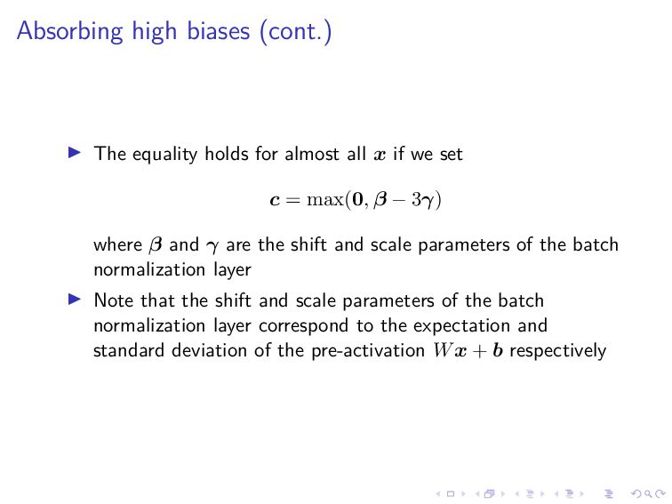
19. Absorbing high biases (cont.) The equality holds for almost all x if we set c = max(0, β − 3γ) where β and γ are the shift and scale parameters of the batch normalization layer Note that the shift and scale parameters of the batch normalization layer correspond to the expectation and standard deviation of the pre-activation Wx + b respectively
20. Experimental results cited from Nagel et al. (2019)
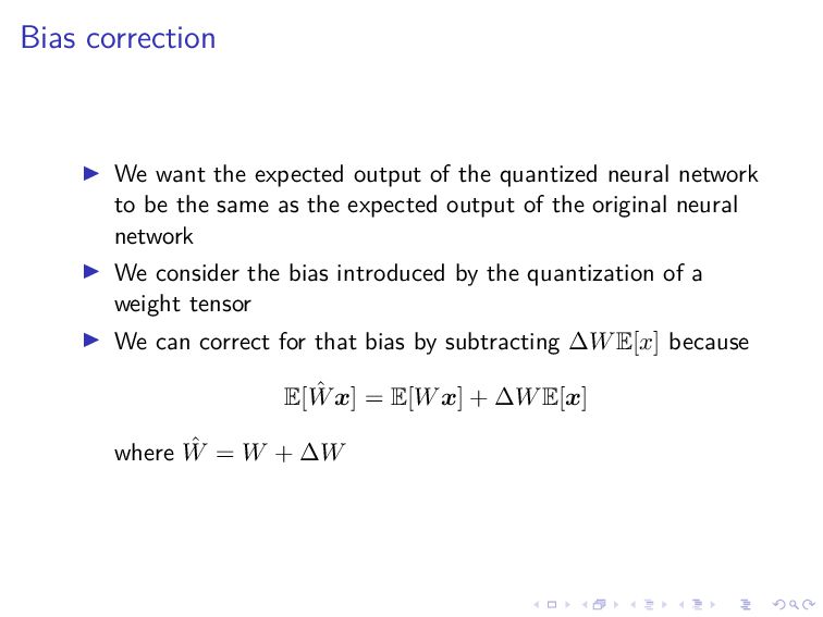
21. Bias correction We want the expected output of the quantized neural network to be the same as the expected output of the original neural network We consider the bias introduced by the quantization of a weight tensor We can correct for that bias by subtracting ∆WE[x] because E[ ˆ Wx] = E[Wx] + ∆WE[x] where ˆ W = W + ∆W
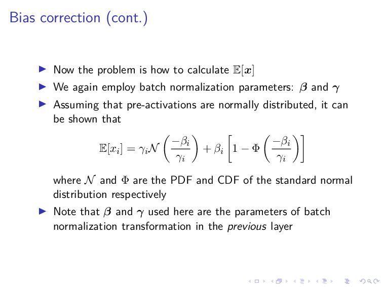
22. Bias correction (cont.) Now the problem is how to calculate E[x] We again employ batch normalization parameters: β and γ Assuming that pre-activations are normally distributed, it can be shown that E[xi] = γiN −βi γi + βi 1 − Φ −βi γi where N and Φ are the PDF and CDF of the standard normal distribution respectively Note that β and γ used here are the parameters of batch normalization transformation in the previous layer
23. Experimental results cited from Nagel et al. (2019)
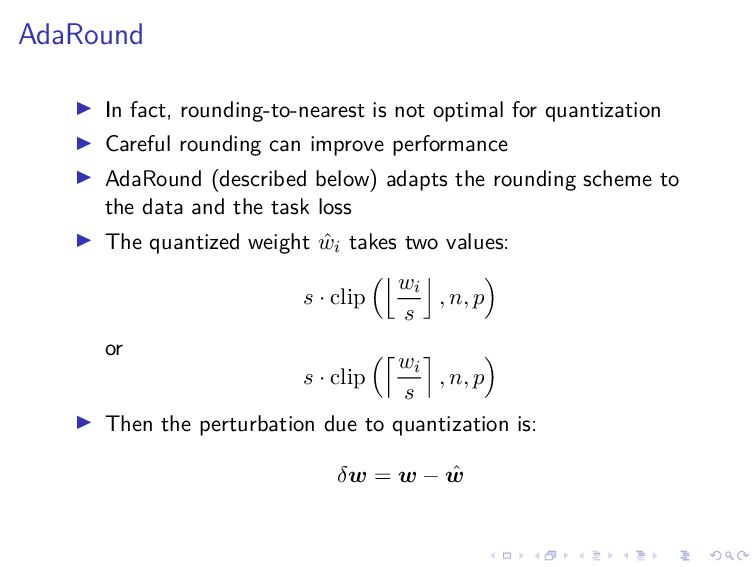
24. AdaRound In fact, rounding-to-nearest is not optimal for quantization Careful rounding can improve performance AdaRound (described below) adapts the rounding scheme to the data and the task loss The quantized weight ˆ wi takes two values: s · clip wi s , n, p or s · clip wi s , n, p Then the perturbation due to quantization is: δw = w − ˆ w
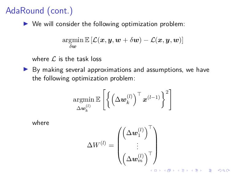
25. AdaRound (cont.) We will consider the following optimization problem: argmin δw E [L(x, y, w + δw) − L(x, y, w)] where L is the task loss By making several approximations and assumptions, we have the following optimization problem: argmin ∆w(l) k E ∆w(l) k x(l−1) 2 where ∆W(l) =      ∆w(l) 1 . . . ∆w(l) m     
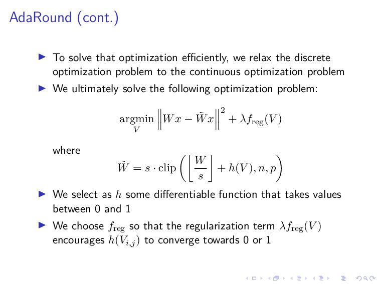
26. AdaRound (cont.) To solve that optimization efficiently, we relax the discrete optimization problem to the continuous optimization problem We ultimately solve the following optimization problem: argmin V Wx − ˜ Wx 2 + λfreg(V ) where ˜ W = s · clip W s + h(V ), n, p We select as h some differentiable function that takes values between 0 and 1 We choose freg so that the regularization term λfreg(V ) encourages h(Vi,j) to converge towards 0 or 1
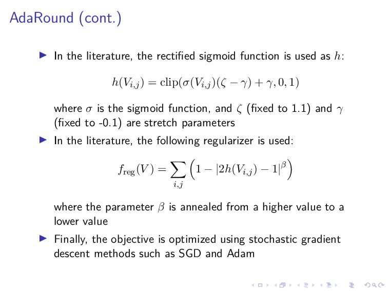
27. AdaRound (cont.) In the literature, the rectified sigmoid function is used as h: h(Vi,j) = clip(σ(Vi,j)(ζ − γ) + γ, 0, 1) where σ is the sigmoid function, and ζ (fixed to 1.1) and γ (fixed to -0.1) are stretch parameters In the literature, the following regularizer is used: freg(V ) = i,j 1 − |2h(Vi,j) − 1|β where the parameter β is annealed from a higher value to a lower value Finally, the objective is optimized using stochastic gradient descent methods such as SGD and Adam
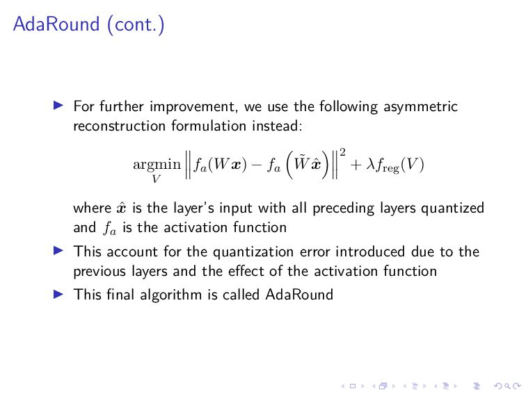
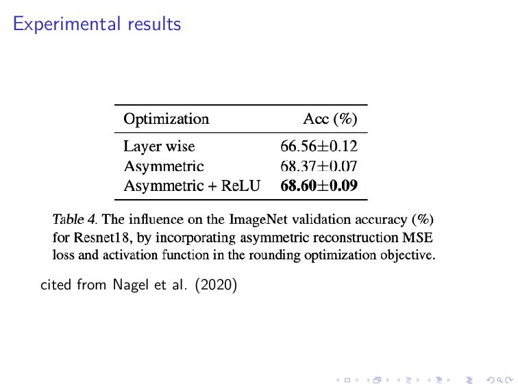
28. AdaRound (cont.) For further improvement, we use the following asymmetric reconstruction formulation instead: argmin V fa(Wx) − fa ˜ W ˆ x 2 + λfreg(V ) where ˆ x is the layer’s input with all preceding layers quantized and fa is the activation function This account for the quantization error introduced due to the previous layers and the effect of the activation function This final algorithm is called AdaRound
29. Experimental results cited from Nagel et al. (2020)
30. Experimental results cited from Nagel et al. (2020)
31. References M. Nagel, M. V. Baalen, T. Blankevoort and M. Welling, ”Data-Free Quantization Through Weight Equalization and Bias Correction,” 2019 IEEE/CVF International Conference on Computer Vision (ICCV), 2019, pp. 1325-1334 Nagel, M., Amjad, R.A., Van Baalen, M., Louizos, C. and Blankevoort, T. (2020). ”Up or Down? Adaptive Rounding for Post-Training Quantization,” Proceedings of the 37th International Conference on Machine Learning Nagel, Markus and Fournarakis, Marios and Amjad, Rana Ali and Bondarenko, Yelysei and van Baalen, Mart and Blankevoort, Tijmen, ”A White Paper on Neural Network Quantization,” arXiv, 2021