OpenTalks.AI - Оселедец Иван, Открытые задачи машинного обучения

Transcript

1. Ivan Oseledets, Skoltech 1 Open problems in machine learning
2. Preamble 2
3. Geometry Score: A Method For Comparing Generative Adversarial Networks Valentin Khrulkov and Ivan Oseledets
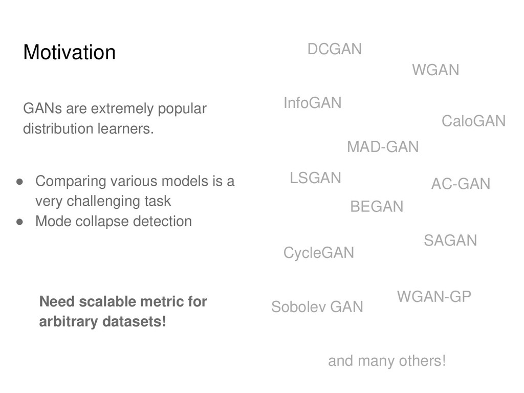
4. Motivation • Comparing various models is a very challenging task • Mode collapse detection LSGAN DCGAN WGAN WGAN-GP SAGAN CycleGAN InfoGAN AC-GAN MAD-GAN CaloGAN BEGAN Sobolev GAN and many others! GANs are extremely popular distribution learners. Need scalable metric for arbitrary datasets!
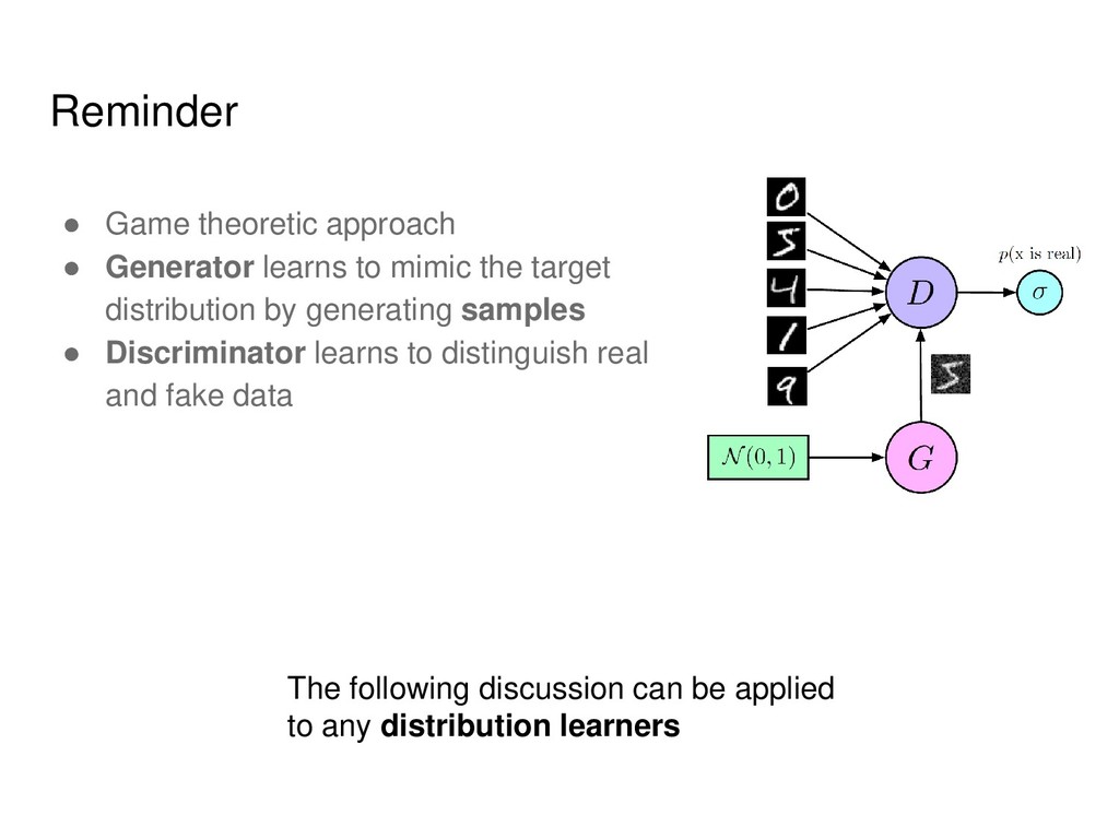
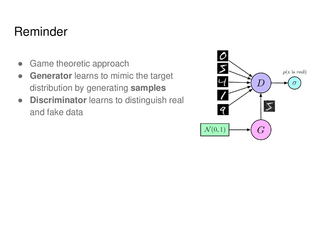
5. Reminder • Game theoretic approach • Generator learns to mimic the target distribution by generating samples • Discriminator learns to distinguish real and fake data The following discussion can be applied to any distribution learners
6. How to assess performance of a GAN? Evaluating the performance of a GAN is difficult - no log likelihood Which one is better? vs
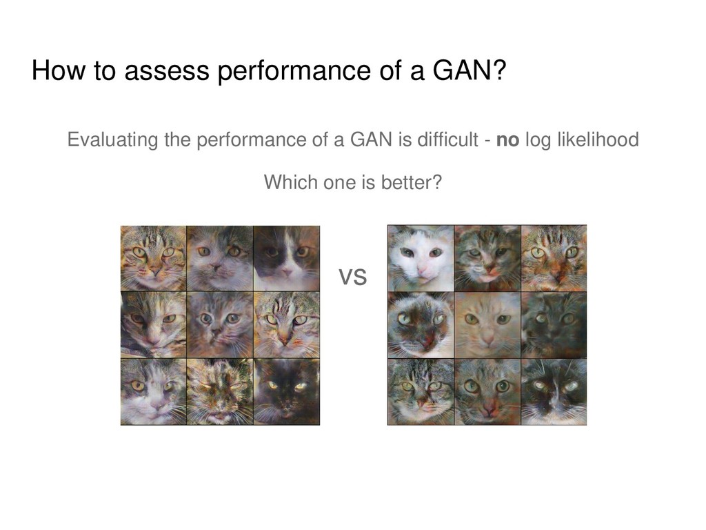
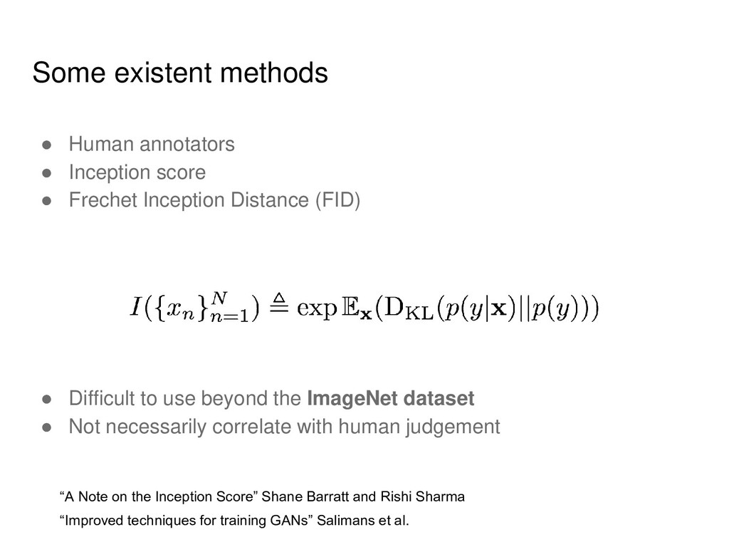
7. Some existent methods • Human annotators • Inception score • Frechet Inception Distance (FID) • Difficult to use beyond the ImageNet dataset • Not necessarily correlate with human judgement “A Note on the Inception Score” Shane Barratt and Rishi Sharma “Improved techniques for training GANs” Salimans et al.
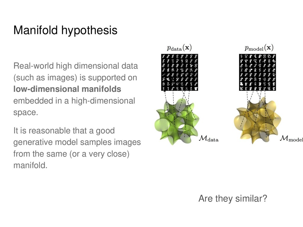
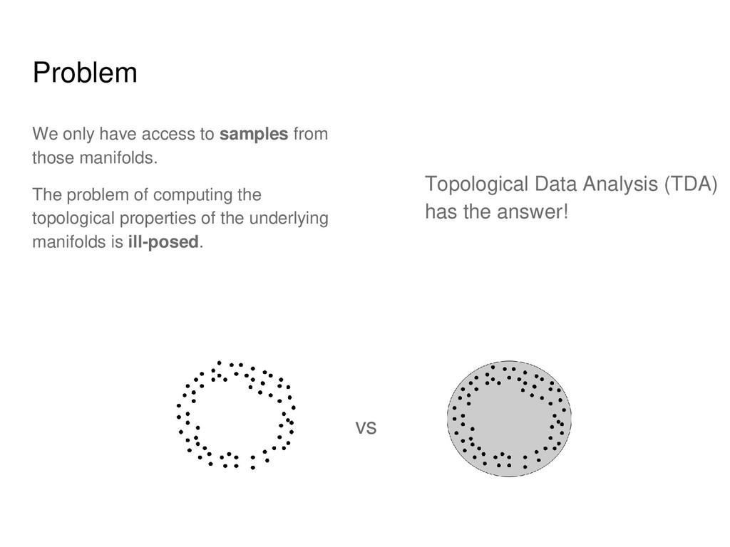
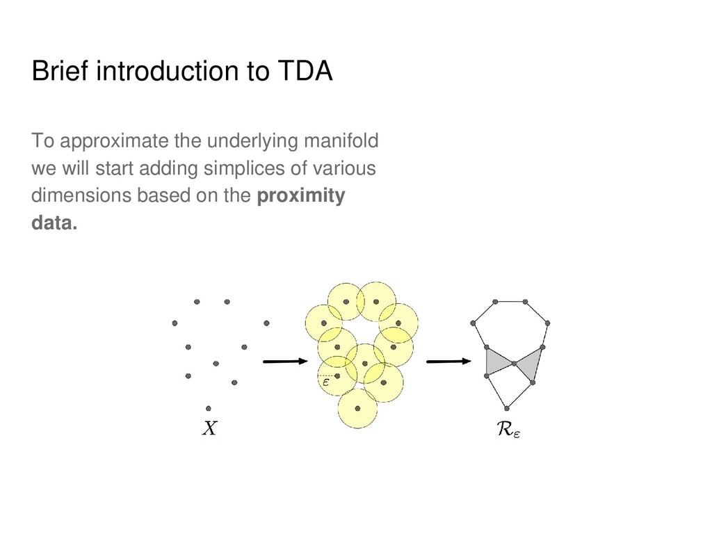
8. Manifold hypothesis Real-world high dimensional data (such as images) is supported on low-dimensional manifolds embedded in a high-dimensional space. It is reasonable that a good generative model samples images from the same (or a very close) manifold. Are they similar?
9. Reminder • Game theoretic approach • Generator learns to mimic the target distribution by generating samples • Discriminator learns to distinguish real and fake data
10. Our idea We use topological properties of the generated and of the data manifolds to measure their similarity. I.e. the manifolds may not coincide precisely, but we want them to have the same shape. Mathematical tool that can be used to describe shape is homology. Also, it can be rather easily computed.
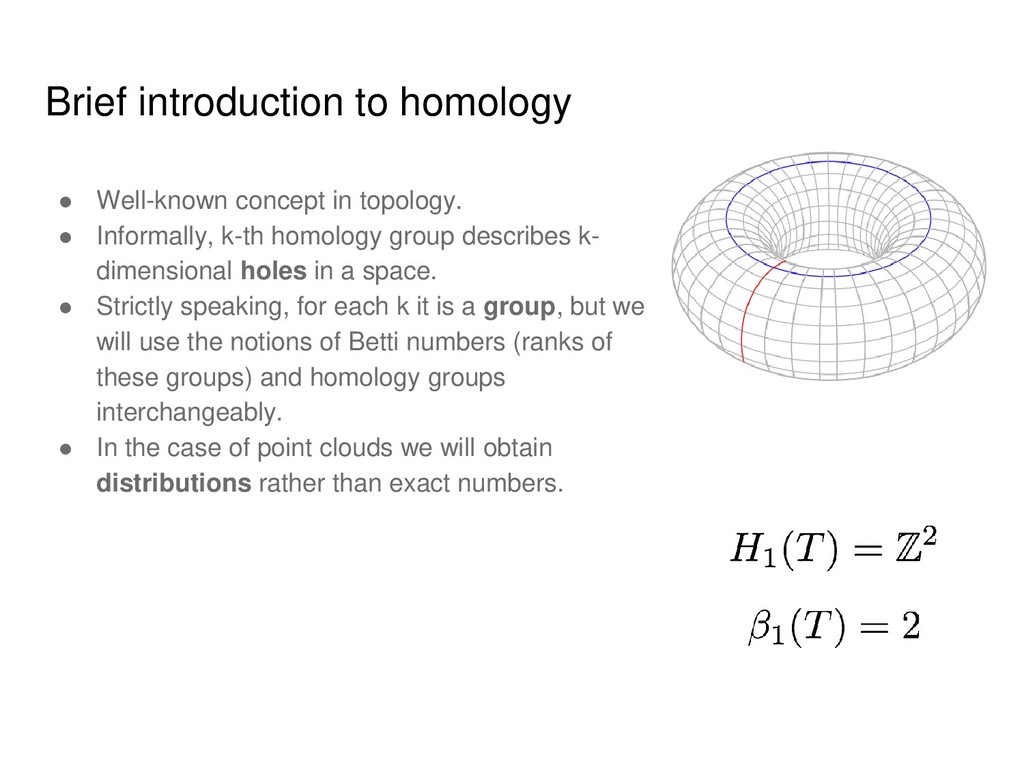
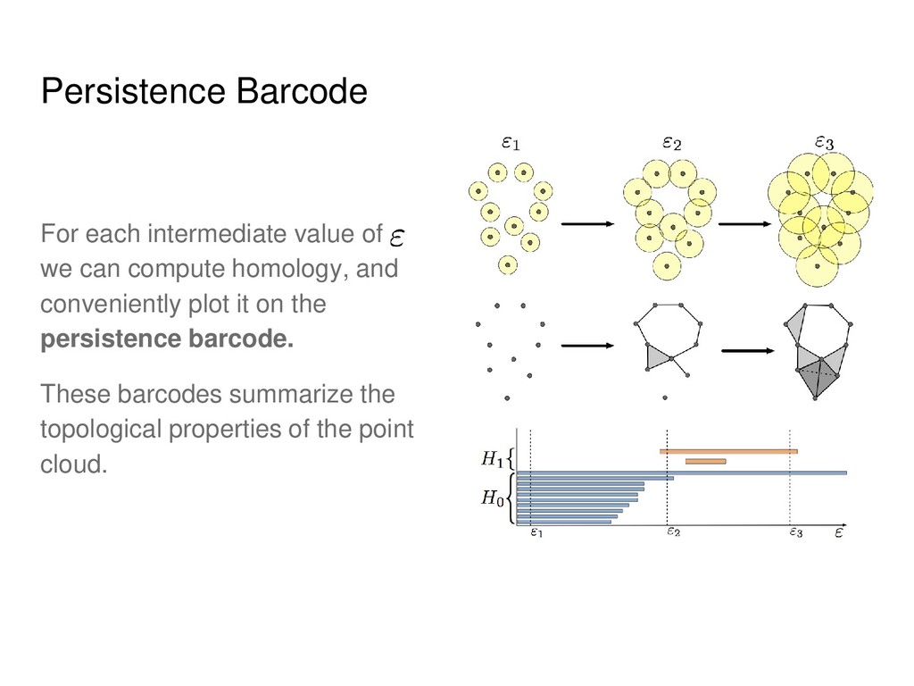
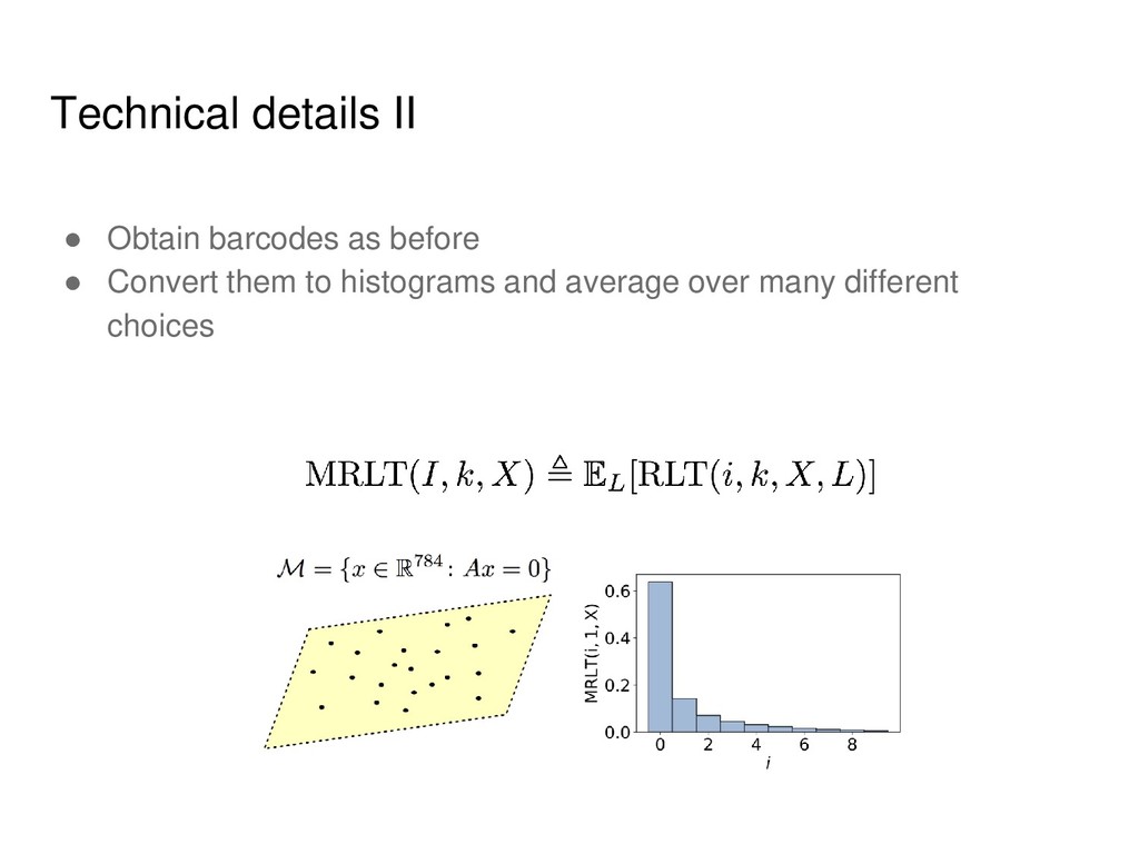
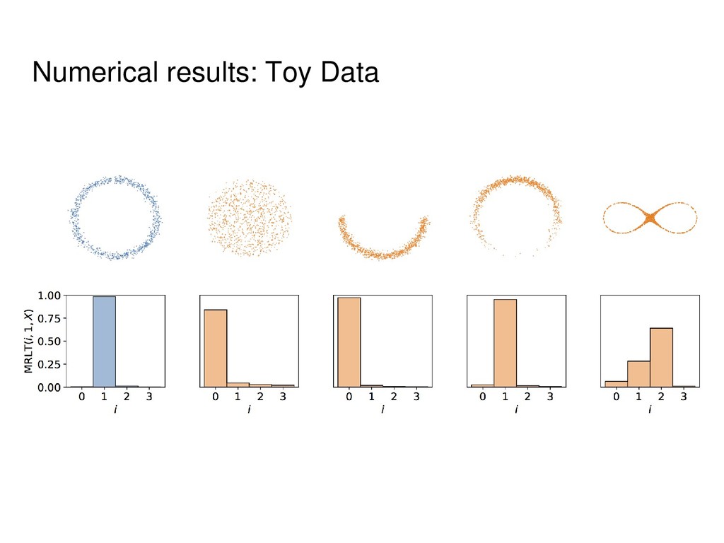
11. Brief introduction to homology • Well-known concept in topology. • Informally, k-th homology group describes k- dimensional holes in a space. • Strictly speaking, for each k it is a group, but we will use the notions of Betti numbers (ranks of these groups) and homology groups interchangeably. • In the case of point clouds we will obtain distributions rather than exact numbers.
12. Problem We only have access to samples from those manifolds. The problem of computing the topological properties of the underlying manifolds is ill-posed. Topological Data Analysis (TDA) has the answer! vs
13. Brief introduction to TDA To approximate the underlying manifold we will start adding simplices of various dimensions based on the proximity data.
14. Persistence Barcode For each intermediate value of we can compute homology, and conveniently plot it on the persistence barcode. These barcodes summarize the topological properties of the point cloud.
15. What to compare? In principle we can compare these barcodes, but this is nontrivial. For each we convert the corresponding piece of the barcode to histograms which can be easily compared.
16. Relative Living Times
17. Technical details II • Obtain barcodes as before • Convert them to histograms and average over many different choices
18. Numerical results: Toy Data
19. Numerical results: MNIST
20. Numerical results: CelebA
21. Numerical results: GANs in particle physics We can also apply this algorithm to datasets of nature other than images.
22. Art of singular vectors and universal adversarial perturbations Valentin Khrulkov and Ivan Oseledets
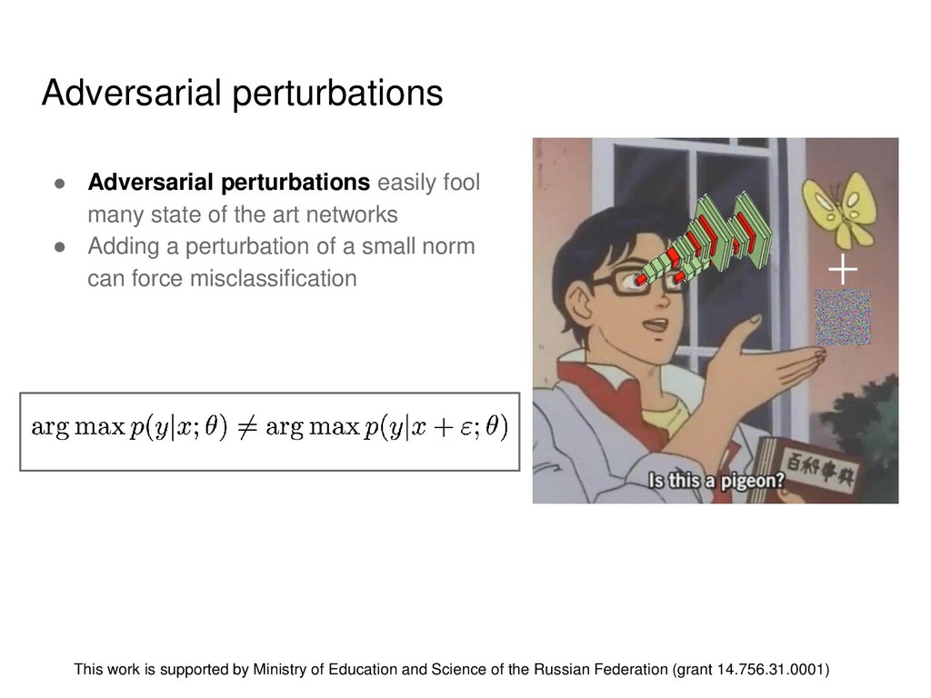
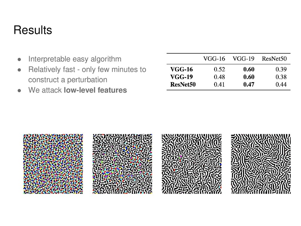
23. Adversarial perturbations • Adversarial perturbations easily fool many state of the art networks • Adding a perturbation of a small norm can force misclassification This work is supported by Ministry of Education and Science of the Russian Federation (grant 14.756.31.0001)
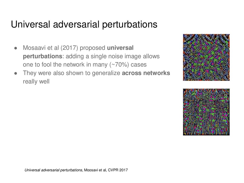
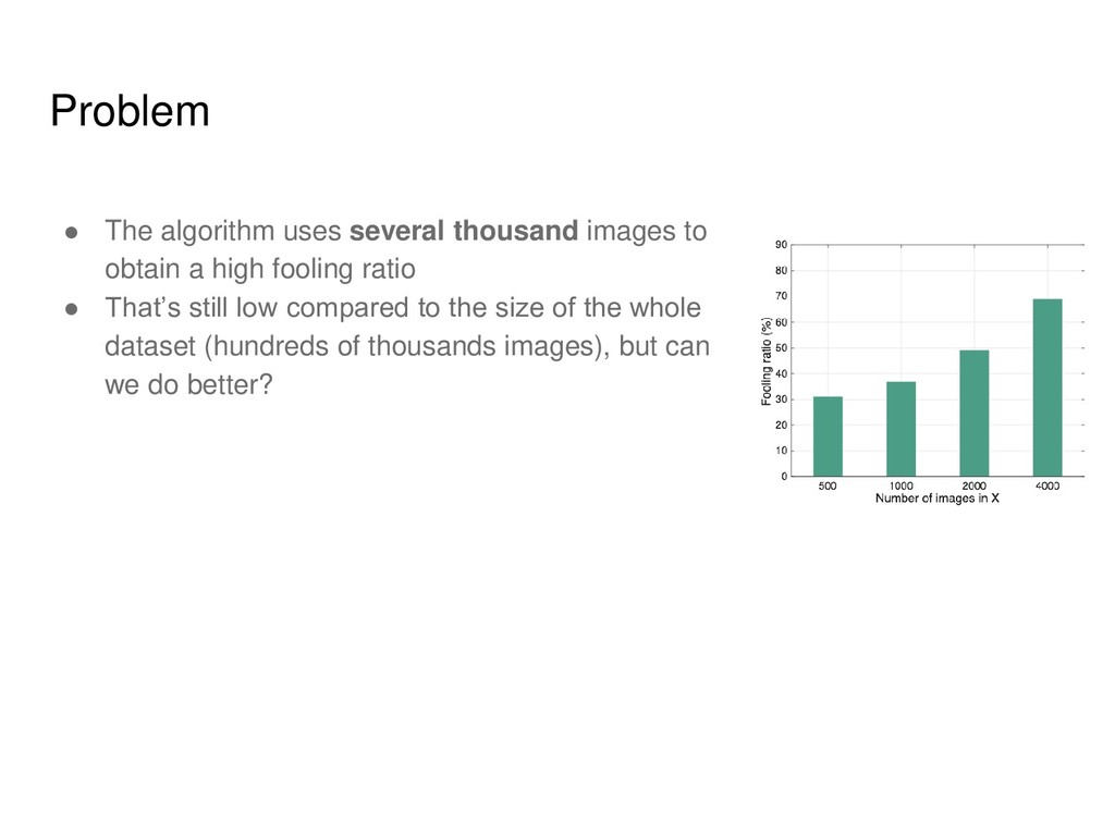
24. Universal adversarial perturbations • Mosaavi et al (2017) proposed universal perturbations: adding a single noise image allows one to fool the network in many (~70%) cases • They were also shown to generalize across networks really well Universal adversarial perturbations, Moosavi et al, CVPR 2017
25. Problem • The algorithm uses several thousand images to obtain a high fooling ratio • That’s still low compared to the size of the whole dataset (hundreds of thousands images), but can we do better?
26. Idea: Let us attack the layers • Goodfellow: linearize the loss (FGSM) • Our idea: linearize a hidden layer
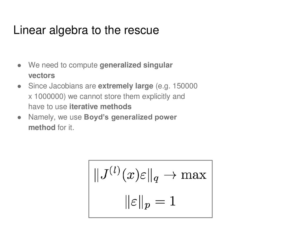
27. Linear algebra to the rescue • We need to compute generalized singular vectors • Since Jacobians are extremely large (e.g. 150000 x 1000000) we cannot store them explicitly and have to use iterative methods • Namely, we use Boyd’s generalized power method for it.
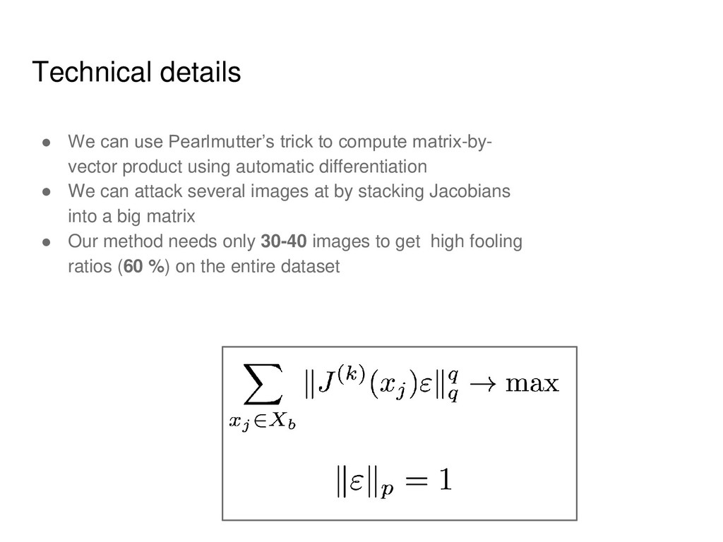
28. Technical details • We can use Pearlmutter’s trick to compute matrix-by- vector product using automatic differentiation • We can attack several images at by stacking Jacobians into a big matrix • Our method needs only 30-40 images to get high fooling ratios (60 %) on the entire dataset
29. Results • Interpretable easy algorithm • Relatively fast - only few minutes to construct a perturbation • We attack low-level features
30. Statistical machine learning • Expressive power - generalization - optimization • No theory for Deep Learning
31. Classical case Number of parameters Approximation Estimation Increases Decreases
32. Deep learning Number of parameters Approximation Estimation Increases Decreases
33. Rethinking generalization Zhang et. al, ICLR 2017 Neural network can remember random labels! 33
34. Deep networks outperform shallow ones
35. Shallow net Deep net Expressive power of CNNs [Nadav Cohen et al., “On the Expressive Power of Deep Learning: A Tensor Analysis”, 2015]
36. Multiplicative RNNs Yuhuai Wu et al. proposed multiplicative RNNs [Y. Wu, S. Zhang, Y. Zhang, Y. Bengio, R. Salakhutdinov., “On Multiplicative Integration with Recurrent Neural Networks”, 2016]
37. Tensor Train RNNs • Simplify: get rid of non- linearity • Generalise: combine W and U into bilinear form T, which is defined a 3d tensor G
38. Tensor Train RNNs • Simplify: get rid of non- linearity • Generalise: combine W and U into bilinear form T, which is defined a 3d tensor G wher e is in the TT- format • Got with shared factors G
39. Tensor perspective • Some form of RNNs • Shallow net (e.g. one conv + global product pooling) TT- decomposition Canonical decomposition
40. Tensor perspective • Shallow net (e.g. one conv + global product pooling) Canonical decomposition
41. Tensor perspective • Some form of RNNs • Shallow net (e.g. one conv + global product pooling) TT- decomposition Canonical decomposition
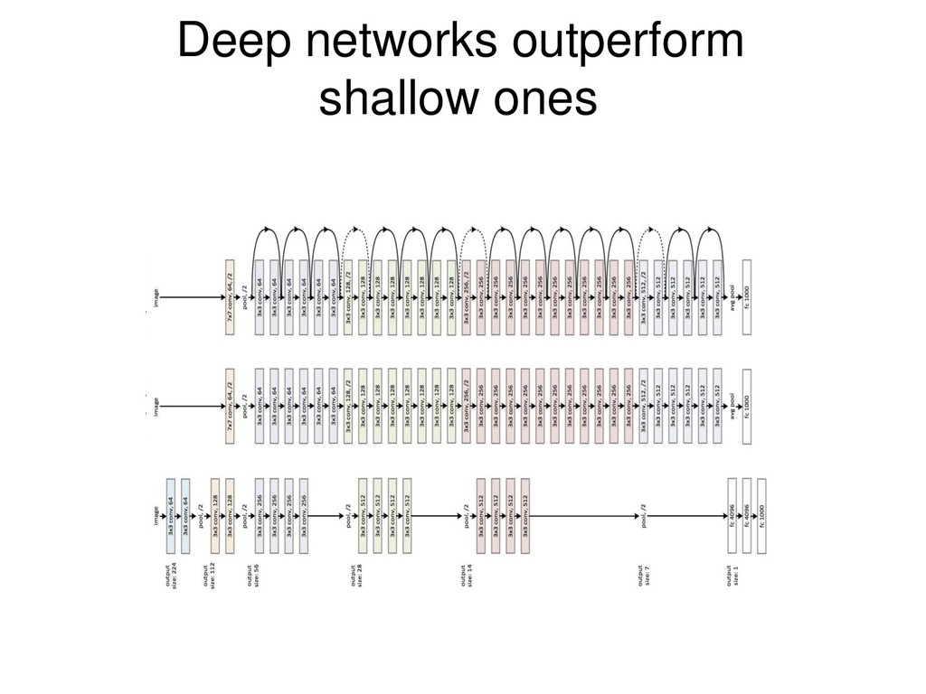
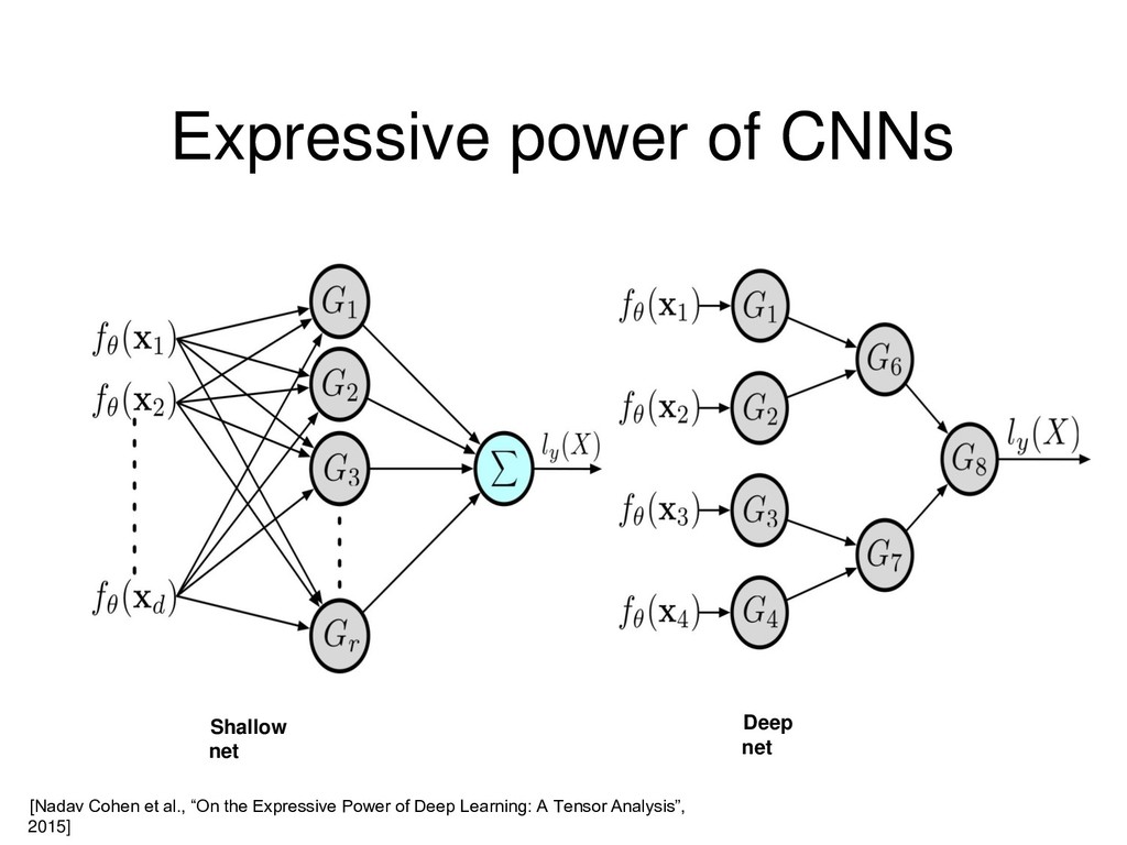
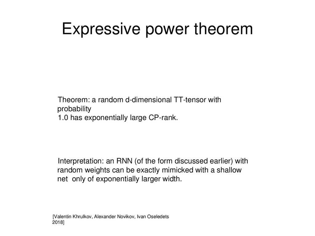
42. Expressive power theorem Theorem: a random d-dimensional TT-tensor with probability 1.0 has exponentially large CP-rank. Interpretation: an RNN (of the form discussed earlier) with random weights can be exactly mimicked with a shallow net only of exponentially larger width. [Valentin Khrulkov, Alexander Novikov, Ivan Oseledets 2018]
43. Feature maps
44. Experiments
45. Quadrature-based features for kernel approximation Marina Munkhoeva, Yermek Kapushev, Evgeny Burnaev and Ivan Oseledets
46. Kernel approximation - Kernel trick: replace scalar products with - Provides good quality for many problems - Scales badly with the number of samples
47. Kernel approximation - Revert the trick: - Use linear methods in the mapped space - How to generate the mapping?
48. Integral representation
49. Integral representation - Shift-invariant kernels - Pointwise nonlinear kernels
50. Random Fourier Features [Rachimi and Recht, 2008] Introduced random Fourier Features (RFF) for any shift-invariant kernel Just Monte-Carlo for the integral!
51. Better quadratures
52. Better quadratures
54. Reinforcement learning Agent knows nothing about the system 54
55. Reinforcement learning RL agent are better than human in many games 55
56. NIPS 2018 AI for prosthetics challenge Make human walk in very accurate simulator 56
57. NIPS 2018 AI for prosthetics challenge 300+ participants 4500+ solutions Our Russian team- 3 place 57
58. Problems not discussed 58 - Optimal experiment design - Importance sampling for stochastic optimization methods