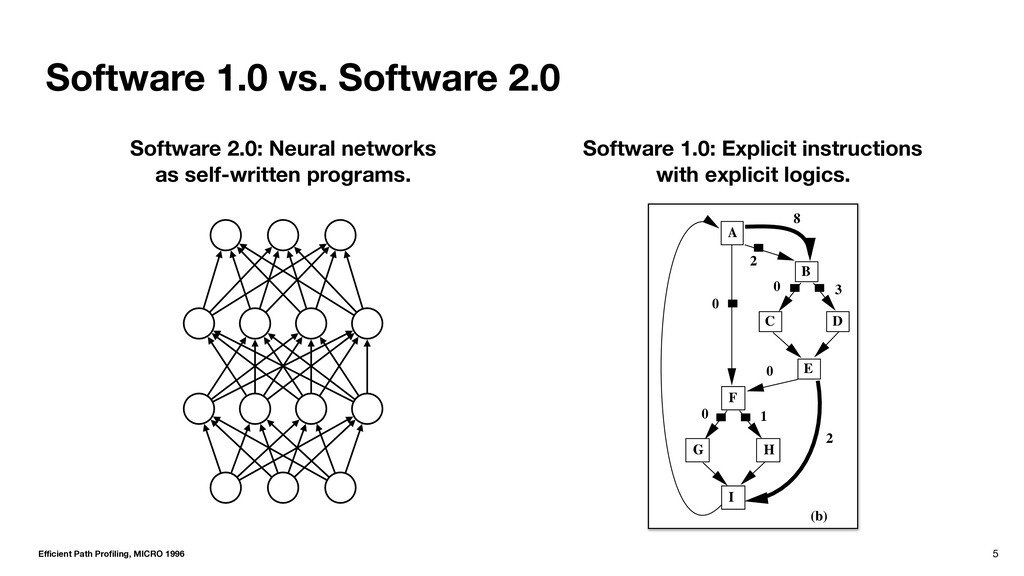
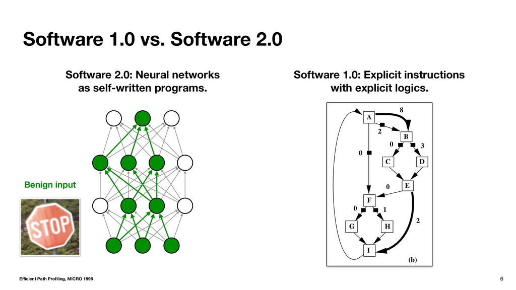
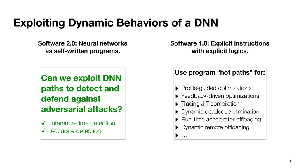
F C E B D r=0 count[r]++ r=0; count[r]++ 1 2 4 A I G H F C E B D 1 2 0 0 0 3 0 2 8 (a) (b) Apply th (Section increme The dumm , whic count. The du responds to r backedge. T corre the backedge Figure 10 and edge val edges. As a guish the fou Software 2.0: Neural networks as self-written programs. Software 1.0: Explicit instructions with explicit logics. Efficient Path Profiling, MICRO 1996
F C E B D r=0 count[r]++ r=0; count[r]++ 1 2 4 A I G H F C E B D 1 2 0 0 0 3 0 2 8 (a) (b) Apply th (Section increme The dumm , whic count. The du responds to r backedge. T corre the backedge Figure 10 and edge val edges. As a guish the fou Software 2.0: Neural networks as self-written programs. Software 1.0: Explicit instructions with explicit logics. Efficient Path Profiling, MICRO 1996 Benign input
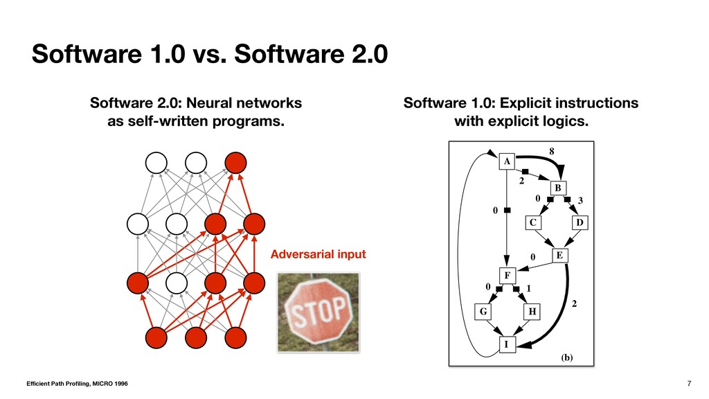
F C E B D r=0 count[r]++ r=0; count[r]++ 1 2 4 A I G H F C E B D 1 2 0 0 0 3 0 2 8 (a) (b) Apply th (Section increme The dumm , whic count. The du responds to r backedge. T corre the backedge Figure 10 and edge val edges. As a guish the fou Software 2.0: Neural networks as self-written programs. Software 1.0: Explicit instructions with explicit logics. Efficient Path Profiling, MICRO 1996 Adversarial input
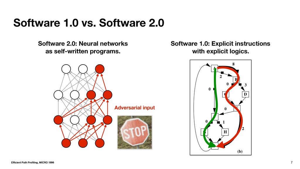
F C E B D r=0 count[r]++ r=0; count[r]++ 1 2 4 A I G H F C E B D 1 2 0 0 0 3 0 2 8 (a) (b) Apply th (Section increme The dumm , whic count. The du responds to r backedge. T corre the backedge Figure 10 and edge val edges. As a guish the fou Software 2.0: Neural networks as self-written programs. Software 1.0: Explicit instructions with explicit logics. Efficient Path Profiling, MICRO 1996 Adversarial input
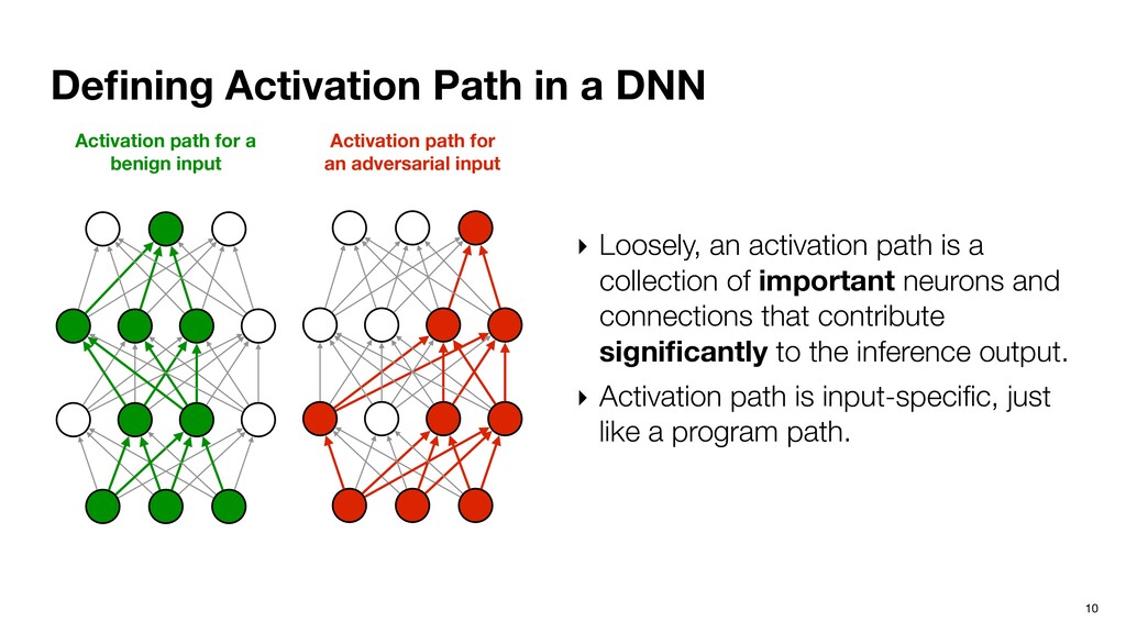
activation path is a collection of important neurons and connections that contribute significantly to the inference output. ‣ Activation path is input-specific, just like a program path. Activation path for a benign input Activation path for an adversarial input
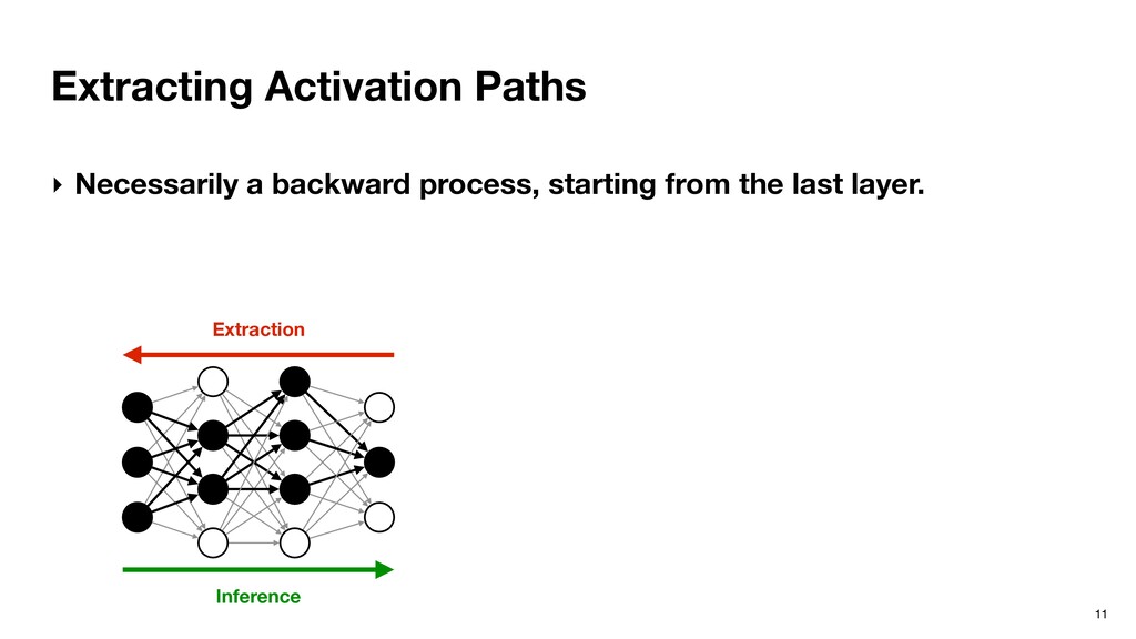
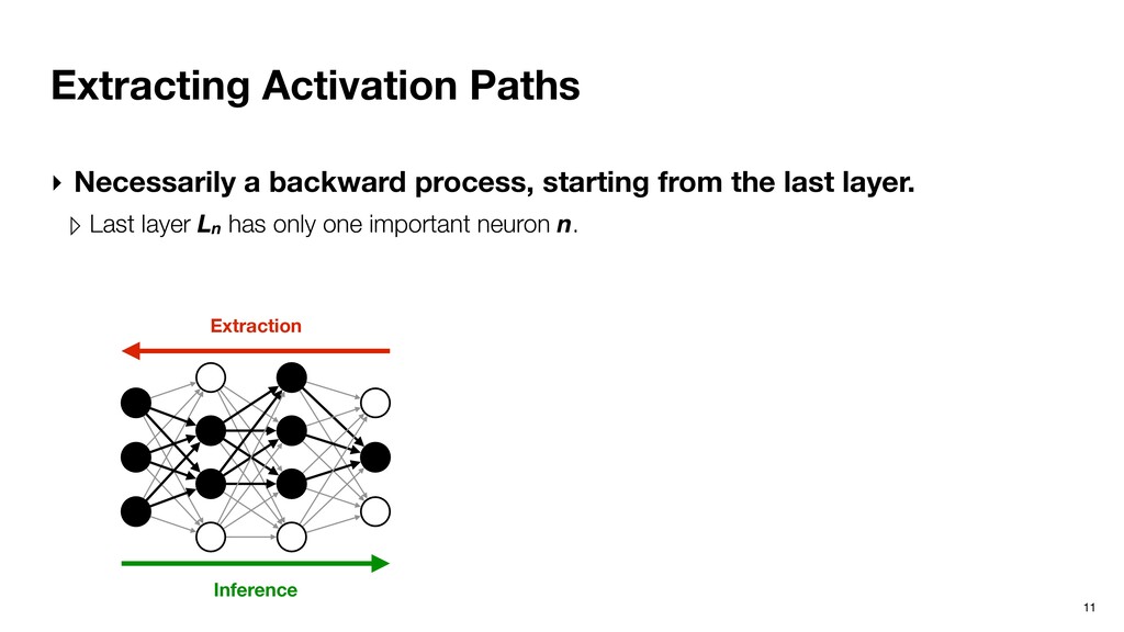
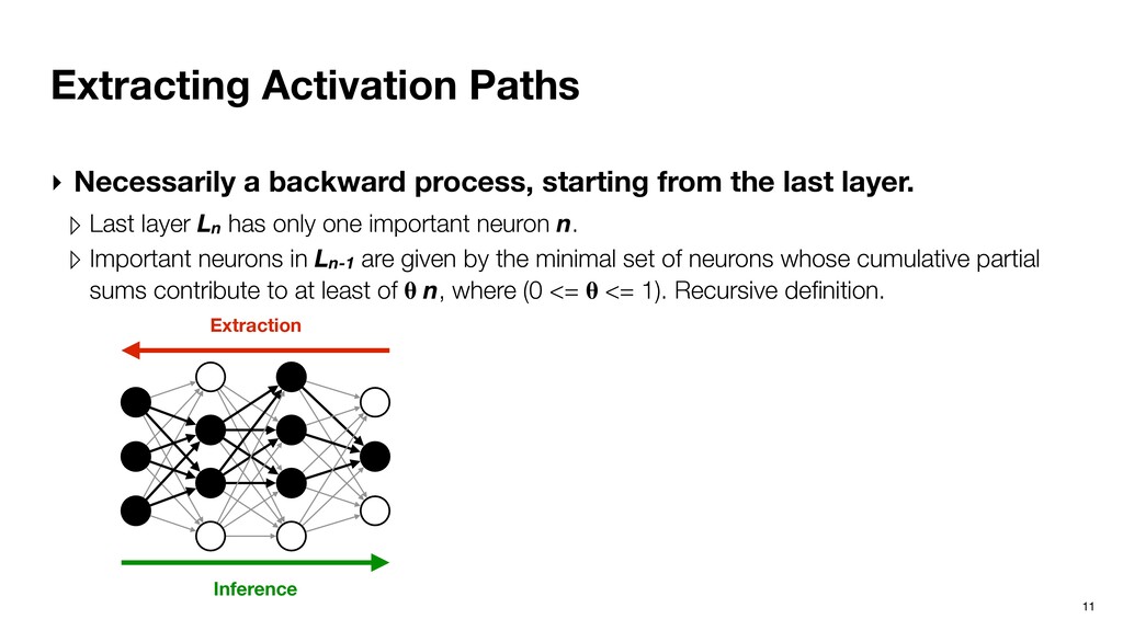
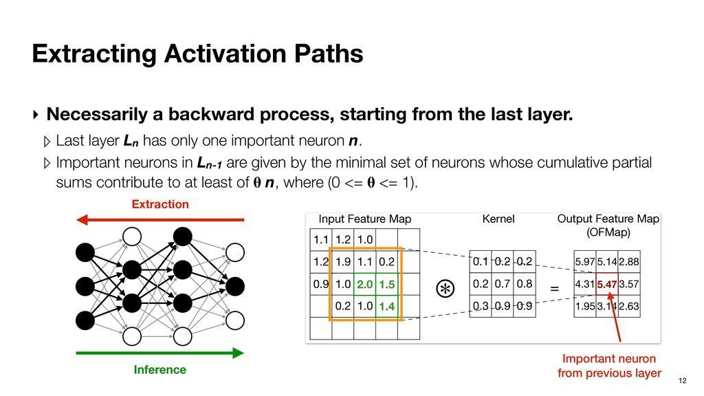
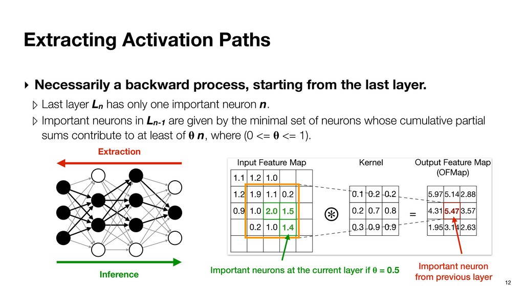
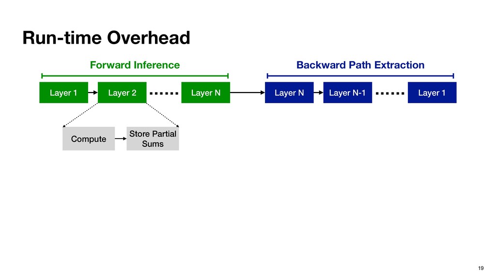
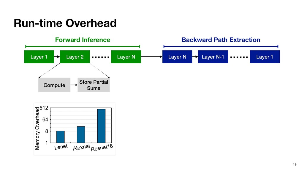
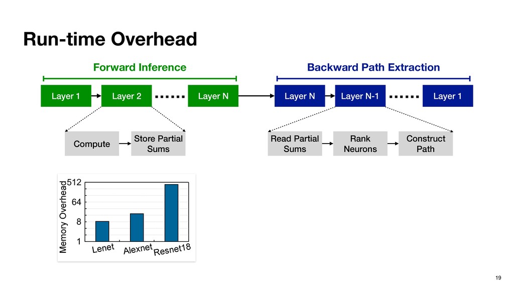
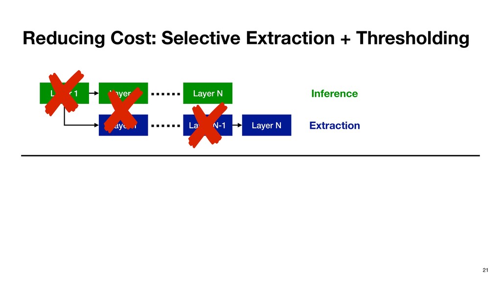
from the last layer. ▹ Last layer Ln has only one important neuron n. ▹ Important neurons in Ln-1 are given by the minimal set of neurons whose cumulative partial sums contribute to at least of n, where (0 <= <= 1). Recursive definition. Inference Extraction
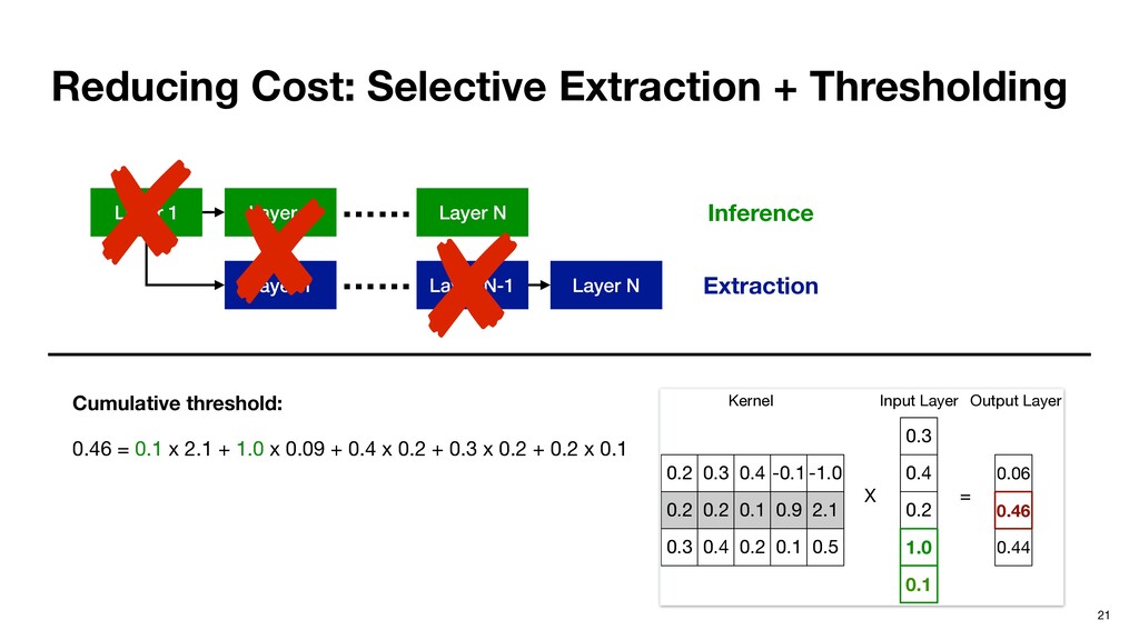
from the last layer. ▹ Last layer Ln has only one important neuron n. ▹ Important neurons in Ln-1 are given by the minimal set of neurons whose cumulative partial sums contribute to at least of n, where (0 <= <= 1). Recursive definition. 0.3 0.4 0.2 1.0 0.1 0.2 0.2 0.3 0.3 0.2 0.4 0.4 0.1 0.2 -0.1 0.9 0.1 -1.0 2.1 0.5 0.06 0.44 = X 0.46 Input Layer Kernel Output Layer Inference Extraction
from the last layer. ▹ Last layer Ln has only one important neuron n. ▹ Important neurons in Ln-1 are given by the minimal set of neurons whose cumulative partial sums contribute to at least of n, where (0 <= <= 1). Recursive definition. 0.3 0.4 0.2 1.0 0.1 0.2 0.2 0.3 0.3 0.2 0.4 0.4 0.1 0.2 -0.1 0.9 0.1 -1.0 2.1 0.5 0.06 0.44 = X 0.46 Input Layer Kernel Output Layer Inference Extraction Important neuron from previous layer
from the last layer. ▹ Last layer Ln has only one important neuron n. ▹ Important neurons in Ln-1 are given by the minimal set of neurons whose cumulative partial sums contribute to at least of n, where (0 <= <= 1). Recursive definition. 0.3 0.4 0.2 1.0 0.1 0.2 0.2 0.3 0.3 0.2 0.4 0.4 0.1 0.2 -0.1 0.9 0.1 -1.0 2.1 0.5 0.06 0.44 = X 0.46 Input Layer Kernel Output Layer Inference Extraction Important neurons at the current layer if = 0.5 Important neuron from previous layer
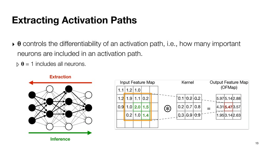
from the last layer. ▹ Last layer Ln has only one important neuron n. ▹ Important neurons in Ln-1 are given by the minimal set of neurons whose cumulative partial sums contribute to at least of n, where (0 <= <= 1). 0.3 0.4 0.2 1.0 0.1 0.2 0.2 0.3 0.3 0.2 0.4 0.4 0.1 0.2 -0.1 0.09 0.1 -1.0 2.1 0.5 0.06 0.44 = X 6 = 0.1 x 2.1 + 1.0 x 0.09 + 0.4 x 0.2 + 0.3 x 0.2 + 0.2 x 0.1 x 2.1 + 1.0 x 0.09 > 0.6 x 0.46, assuming θ = 0.6 0.46 t Feature Map Kernel Output Feature Map (OFMap) 2.63 1.1 1.2 0.9 0.2 1.2 1.9 1.0 1.0 1.1 ⊛ 0.1 0.2 0.2 0.7 0.2 1.0 5.97 4.31 1.95 5.14 3.14 2.88 3.57 0.3 0.9 0.2 0.8 0.9 = 5.47 = 2.0 x 0.7 + 1.4 x 0.9 + 1.5 x 0.8 + 1.0 x 0.9 + …… 2.0 x 0.7 + 1.4 x 0.9 + 1.5 x 0.8 > 0.6 x 5.47, assuming θ = 0.6 2.0 1.4 5.47 1.5 Input Feature Map Kernel Output Feature Map (OFMap) Important Neuron Extraction in Fully-connected Layer Important Neuron Extraction in Convolution Layer Const from Inference Extraction
from the last layer. ▹ Last layer Ln has only one important neuron n. ▹ Important neurons in Ln-1 are given by the minimal set of neurons whose cumulative partial sums contribute to at least of n, where (0 <= <= 1). 0.3 0.4 0.2 1.0 0.1 0.2 0.2 0.3 0.3 0.2 0.4 0.4 0.1 0.2 -0.1 0.09 0.1 -1.0 2.1 0.5 0.06 0.44 = X 6 = 0.1 x 2.1 + 1.0 x 0.09 + 0.4 x 0.2 + 0.3 x 0.2 + 0.2 x 0.1 x 2.1 + 1.0 x 0.09 > 0.6 x 0.46, assuming θ = 0.6 0.46 t Feature Map Kernel Output Feature Map (OFMap) 2.63 1.1 1.2 0.9 0.2 1.2 1.9 1.0 1.0 1.1 ⊛ 0.1 0.2 0.2 0.7 0.2 1.0 5.97 4.31 1.95 5.14 3.14 2.88 3.57 0.3 0.9 0.2 0.8 0.9 = 5.47 = 2.0 x 0.7 + 1.4 x 0.9 + 1.5 x 0.8 + 1.0 x 0.9 + …… 2.0 x 0.7 + 1.4 x 0.9 + 1.5 x 0.8 > 0.6 x 5.47, assuming θ = 0.6 2.0 1.4 5.47 1.5 Input Feature Map Kernel Output Feature Map (OFMap) Important Neuron Extraction in Fully-connected Layer Important Neuron Extraction in Convolution Layer Const from Inference Extraction Important neuron from previous layer
from the last layer. ▹ Last layer Ln has only one important neuron n. ▹ Important neurons in Ln-1 are given by the minimal set of neurons whose cumulative partial sums contribute to at least of n, where (0 <= <= 1). 0.3 0.4 0.2 1.0 0.1 0.2 0.2 0.3 0.3 0.2 0.4 0.4 0.1 0.2 -0.1 0.09 0.1 -1.0 2.1 0.5 0.06 0.44 = X 6 = 0.1 x 2.1 + 1.0 x 0.09 + 0.4 x 0.2 + 0.3 x 0.2 + 0.2 x 0.1 x 2.1 + 1.0 x 0.09 > 0.6 x 0.46, assuming θ = 0.6 0.46 t Feature Map Kernel Output Feature Map (OFMap) 2.63 1.1 1.2 0.9 0.2 1.2 1.9 1.0 1.0 1.1 ⊛ 0.1 0.2 0.2 0.7 0.2 1.0 5.97 4.31 1.95 5.14 3.14 2.88 3.57 0.3 0.9 0.2 0.8 0.9 = 5.47 = 2.0 x 0.7 + 1.4 x 0.9 + 1.5 x 0.8 + 1.0 x 0.9 + …… 2.0 x 0.7 + 1.4 x 0.9 + 1.5 x 0.8 > 0.6 x 5.47, assuming θ = 0.6 2.0 1.4 5.47 1.5 Input Feature Map Kernel Output Feature Map (OFMap) Important Neuron Extraction in Fully-connected Layer Important Neuron Extraction in Convolution Layer Const from Inference Extraction Important neurons at the current layer if = 0.5 Important neuron from previous layer
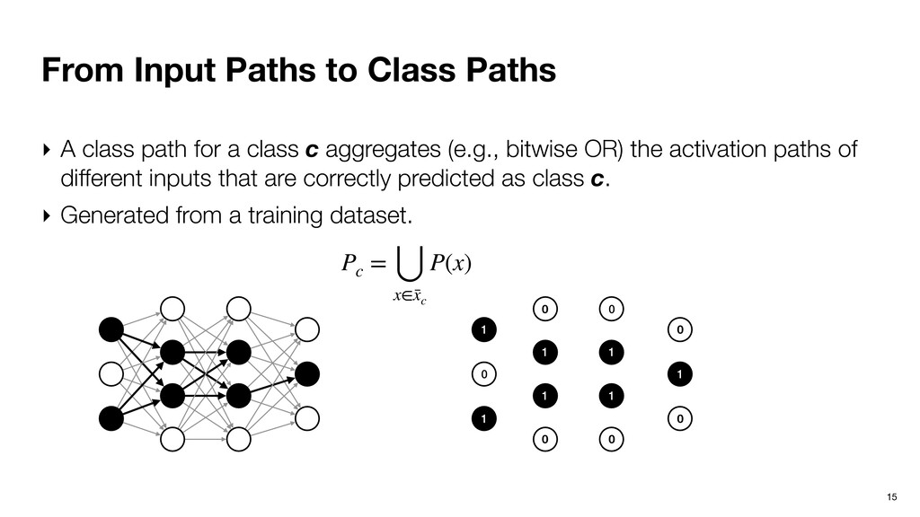
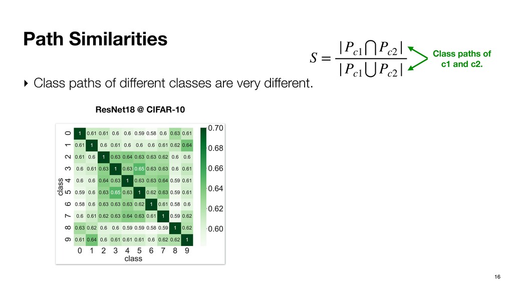
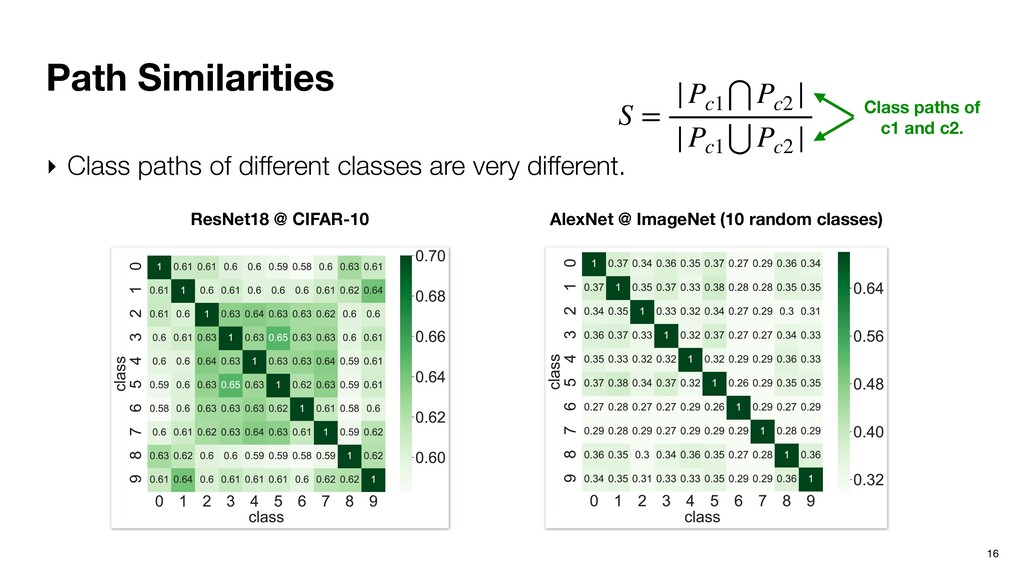
path for a class c aggregates (e.g., bitwise OR) the activation paths of different inputs that are correctly predicted as class c. ‣ Generated from a training dataset. 1 0 1 0 1 1 0 0 1 1 0 0 1 0 Pc = ⋃ x∈¯ xc P(x)
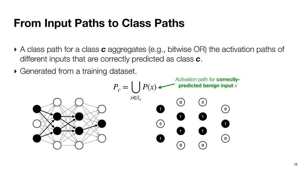
path for a class c aggregates (e.g., bitwise OR) the activation paths of different inputs that are correctly predicted as class c. ‣ Generated from a training dataset. 1 0 1 0 1 1 0 0 1 1 0 0 1 0 Pc = ⋃ x∈¯ xc P(x) Activation path for correctly- predicted benign input x
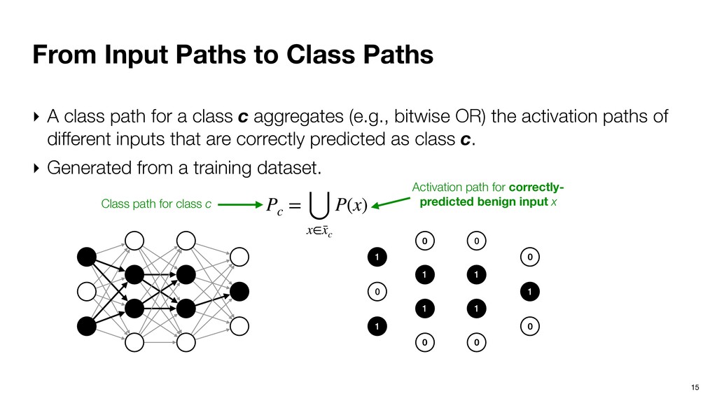
path for a class c aggregates (e.g., bitwise OR) the activation paths of different inputs that are correctly predicted as class c. ‣ Generated from a training dataset. 1 0 1 0 1 1 0 0 1 1 0 0 1 0 Pc = ⋃ x∈¯ xc P(x) Activation path for correctly- predicted benign input x Class path for class c
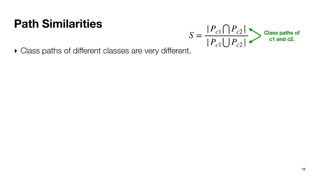
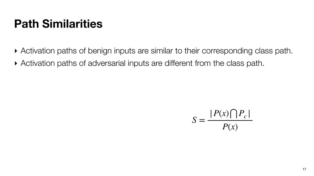
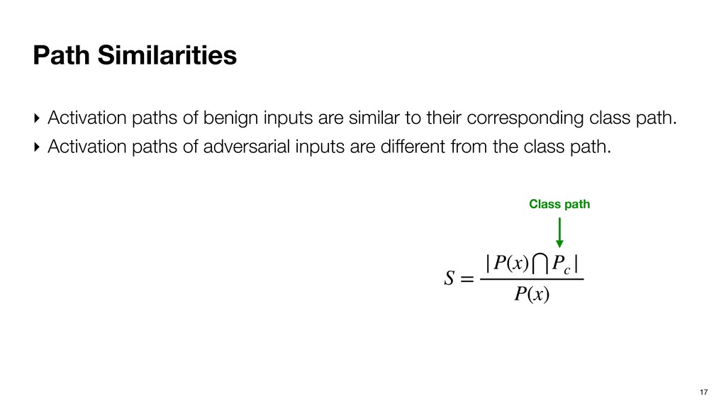
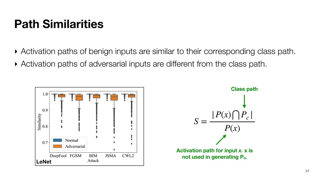
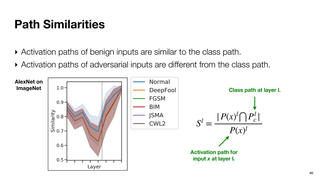
similar to their corresponding class path. ‣ Activation paths of adversarial inputs are different from the class path. S = |P(x)⋂Pc | P(x) Activation path for input x. x is not used in generating Pc. Class path
similar to their corresponding class path. ‣ Activation paths of adversarial inputs are different from the class path. Figure 4: Normal example and perturbations from different attacks. The perturbations are enh the differences. (a) (b) (c) (d) LeNet S = |P(x)⋂Pc | P(x) Activation path for input x. x is not used in generating Pc. Class path
similar to their corresponding class path. ‣ Activation paths of adversarial inputs are different from the class path. Figure 4: Normal example and perturbations from different attacks. The perturbations are enh the differences. (a) (b) (c) (d) LeNet S = |P(x)⋂Pc | P(x) Activation path for input x. x is not used in generating Pc. Class path Benign inputs
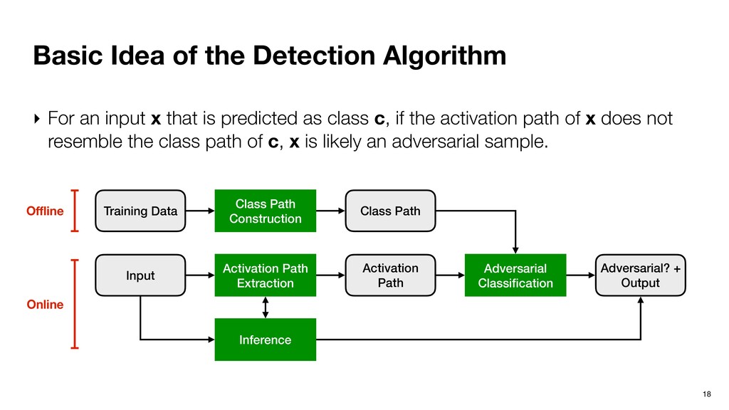
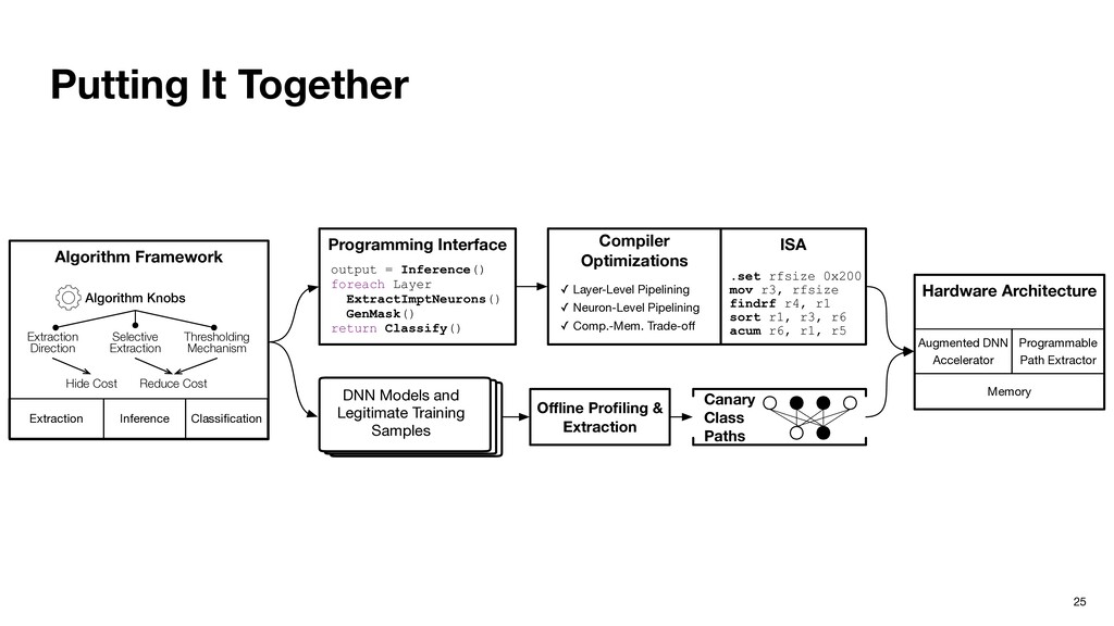
input x that is predicted as class c, if the activation path of x does not resemble the class path of c, x is likely an adversarial sample. Class Path Construction Training Data Class Path Activation Path Extraction Input Inference Adversarial Classification Adversarial? + Output Activation Path Offline Online
input x that is predicted as class c, if the activation path of x does not resemble the class path of c, x is likely an adversarial sample. Class Path Construction Training Data Class Path Activation Path Extraction Input Inference Adversarial Classification Adversarial? + Output Activation Path Offline Online Random forest. Lightweight and works effectively.
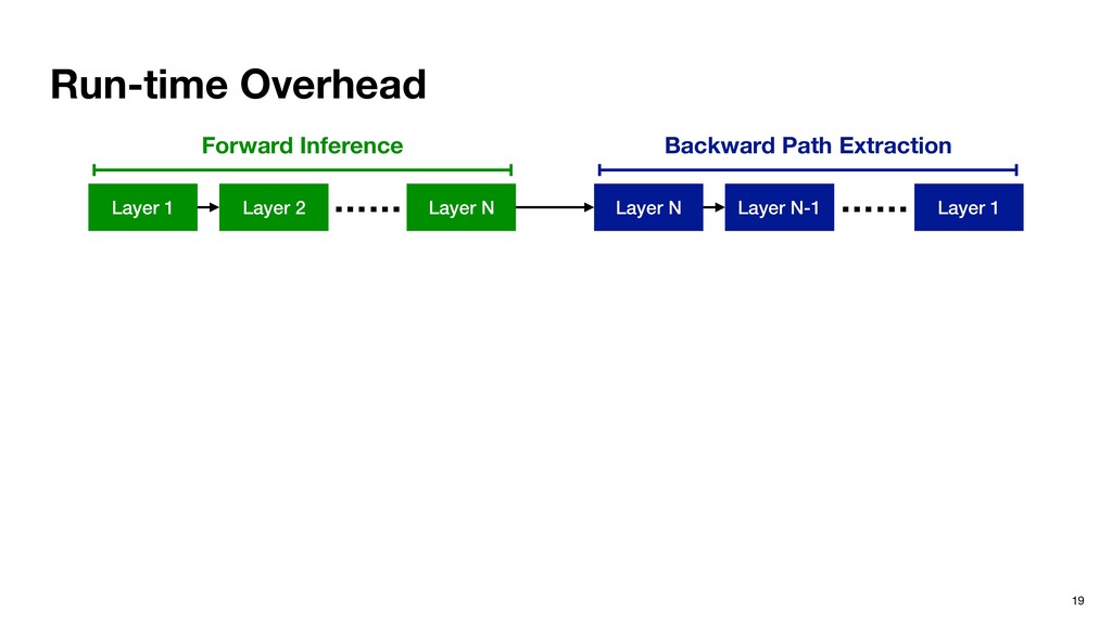
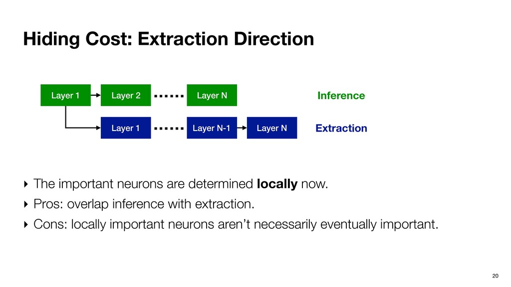
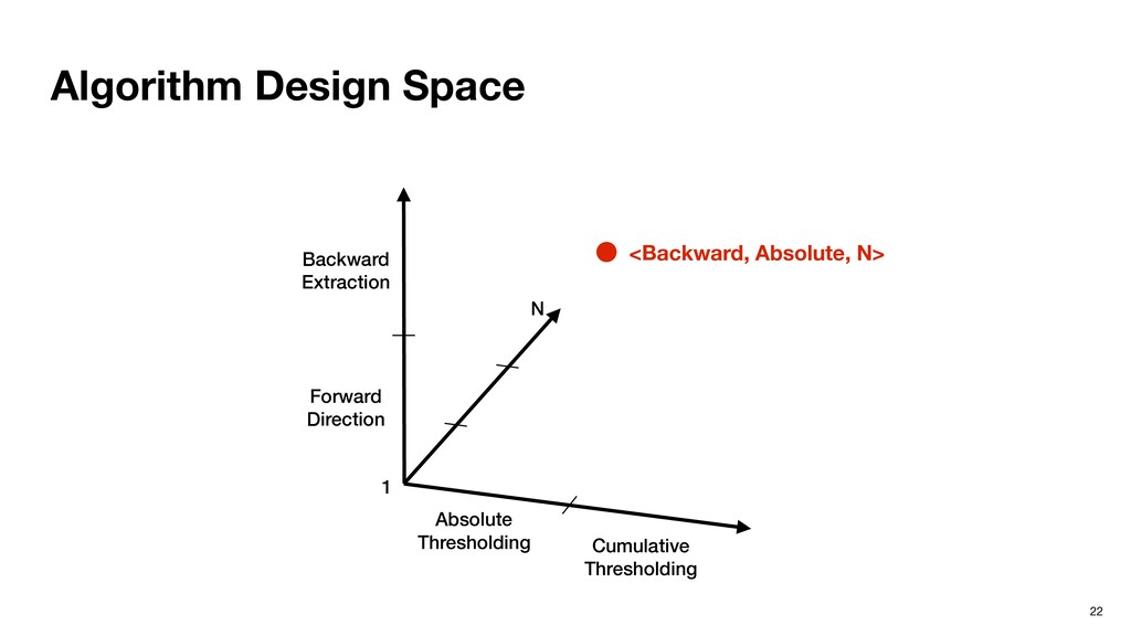
N Layer 1 Layer N-1 Layer N …… …… Inference Extraction ‣ The important neurons are determined locally now. ‣ Pros: overlap inference with extraction. ‣ Cons: locally important neurons aren’t necessarily eventually important.
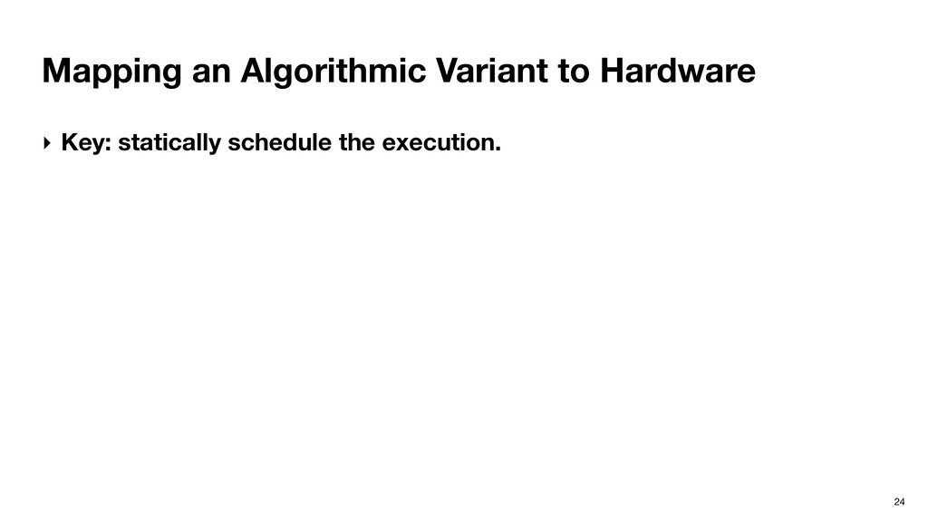
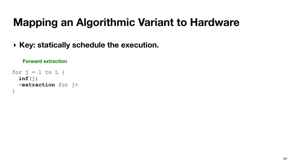
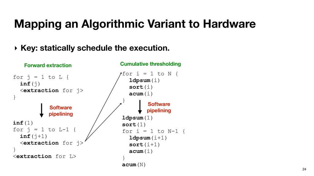
schedule the execution. Forward extraction for j = 1 to L { inf(j) <extraction for j> } Software pipelining inf(1) for j = 1 to L-1 { inf(j+1) <extraction for j> } <extraction for L>
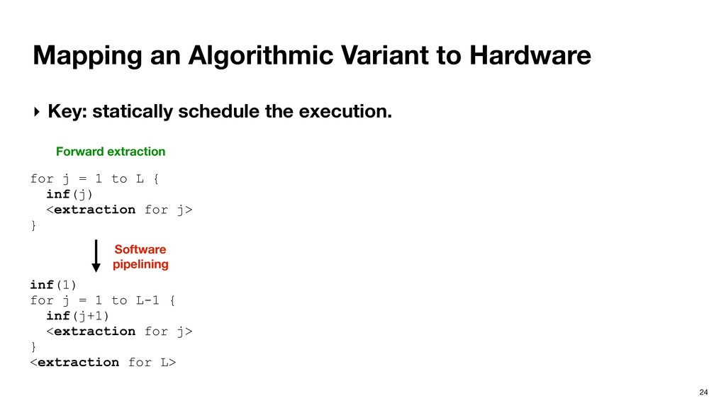
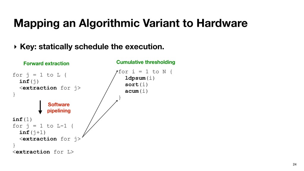
schedule the execution. Forward extraction for j = 1 to L { inf(j) <extraction for j> } Software pipelining inf(1) for j = 1 to L-1 { inf(j+1) <extraction for j> } <extraction for L> Cumulative thresholding for i = 1 to N { ldpsum(i) sort(i) acum(i) }
schedule the execution. Forward extraction for j = 1 to L { inf(j) <extraction for j> } Software pipelining inf(1) for j = 1 to L-1 { inf(j+1) <extraction for j> } <extraction for L> Cumulative thresholding for i = 1 to N { ldpsum(i) sort(i) acum(i) } Software pipelining ldpsum(1) sort(1) for i = 1 to N-1 { ldpsum(i+1) sort(i+1) acum(i) } acum(N)
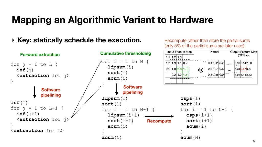
schedule the execution. Forward extraction for j = 1 to L { inf(j) <extraction for j> } 0.3 0.4 0.2 1.0 0.1 0.2 0.2 0.3 0.3 0.2 0.4 0.4 0.1 0.2 -0.1 0.09 0.1 -1.0 2.1 0.5 0.06 0.44 = X 0.46 = 0.1 x 2.1 + 1.0 x 0.09 + 0.4 x 0.2 + 0.3 x 0.2 + 0.2 x 0.1 0.1 x 2.1 + 1.0 x 0.09 > 0.6 x 0.46, assuming θ = 0.6 0.46 Important Neurons identified in the current layer: 1.0, 0.1 Important Neurons in the OFMap (identified before): 0.46 Input Feature Map Kernel Output Feature Map (OFMap) 2.63 1.1 1.2 0.9 0.2 1.2 1.9 1.0 1.0 1.1 ⊛ 0.1 0.2 0.2 0.7 0.2 1.0 5.97 4.31 1.95 5.14 3.14 2.88 3.57 0.3 0.9 0.2 0.8 0.9 = Important Neurons identified in the current layer: 2.0, 1.4, 1.5 Important Neurons in the OFMap (identified before): 5.47 5.47 = 2.0 x 0.7 + 1.4 x 0.9 + 1.5 x 0.8 + 1.0 x 0.9 + …… 2.0 x 0.7 + 1.4 x 0.9 + 1.5 x 0.8 > 0.6 x 5.47, assuming θ = 0.6 2.0 1.4 5.47 1.5 Input Feature Map Kernel Output Feature Map (OFMap) Important Neuron Extraction in Fully-connected Layer Important Neuron Extraction in Convolution Layer C Recompute rather than store the partial sums (only 5% of the partial sums are later used). Software pipelining inf(1) for j = 1 to L-1 { inf(j+1) <extraction for j> } <extraction for L> Cumulative thresholding for i = 1 to N { ldpsum(i) sort(i) acum(i) } Software pipelining ldpsum(1) sort(1) for i = 1 to N-1 { ldpsum(i+1) sort(i+1) acum(i) } acum(N)
schedule the execution. Forward extraction for j = 1 to L { inf(j) <extraction for j> } 0.3 0.4 0.2 1.0 0.1 0.2 0.2 0.3 0.3 0.2 0.4 0.4 0.1 0.2 -0.1 0.09 0.1 -1.0 2.1 0.5 0.06 0.44 = X 0.46 = 0.1 x 2.1 + 1.0 x 0.09 + 0.4 x 0.2 + 0.3 x 0.2 + 0.2 x 0.1 0.1 x 2.1 + 1.0 x 0.09 > 0.6 x 0.46, assuming θ = 0.6 0.46 Important Neurons identified in the current layer: 1.0, 0.1 Important Neurons in the OFMap (identified before): 0.46 Input Feature Map Kernel Output Feature Map (OFMap) 2.63 1.1 1.2 0.9 0.2 1.2 1.9 1.0 1.0 1.1 ⊛ 0.1 0.2 0.2 0.7 0.2 1.0 5.97 4.31 1.95 5.14 3.14 2.88 3.57 0.3 0.9 0.2 0.8 0.9 = Important Neurons identified in the current layer: 2.0, 1.4, 1.5 Important Neurons in the OFMap (identified before): 5.47 5.47 = 2.0 x 0.7 + 1.4 x 0.9 + 1.5 x 0.8 + 1.0 x 0.9 + …… 2.0 x 0.7 + 1.4 x 0.9 + 1.5 x 0.8 > 0.6 x 5.47, assuming θ = 0.6 2.0 1.4 5.47 1.5 Input Feature Map Kernel Output Feature Map (OFMap) Important Neuron Extraction in Fully-connected Layer Important Neuron Extraction in Convolution Layer C Recompute rather than store the partial sums (only 5% of the partial sums are later used). Software pipelining inf(1) for j = 1 to L-1 { inf(j+1) <extraction for j> } <extraction for L> Cumulative thresholding for i = 1 to N { ldpsum(i) sort(i) acum(i) } Software pipelining ldpsum(1) sort(1) for i = 1 to N-1 { ldpsum(i+1) sort(i+1) acum(i) } acum(N) Recompute csps(1) sort(1) for i = 1 to N-1 { csps(i+1) sort(i+1) acum(i) } acum(N)
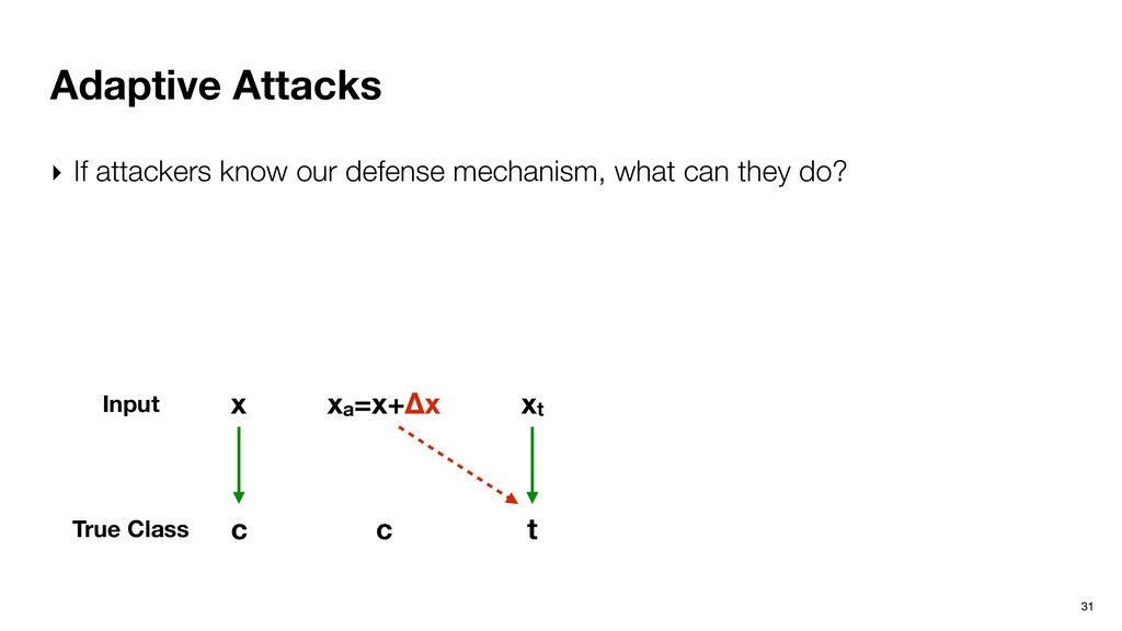
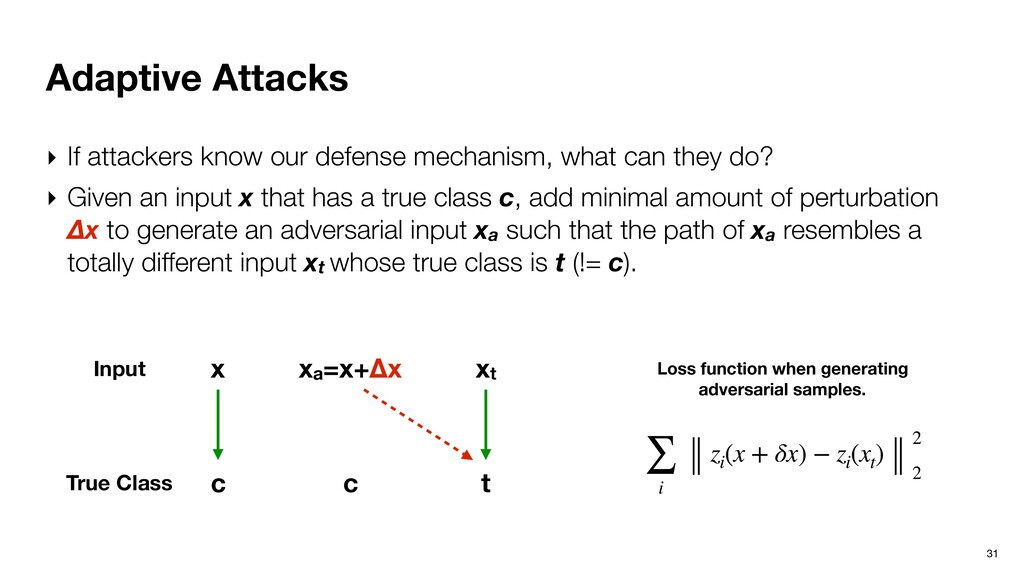
what can they do? ‣ Given an input x that has a true class c, add minimal amount of perturbation Δx to generate an adversarial input xa such that the path of xa resembles a totally different input xt whose true class is t (!= c). x c t Input xt True Class xa=x+Δx c
what can they do? ‣ Given an input x that has a true class c, add minimal amount of perturbation Δx to generate an adversarial input xa such that the path of xa resembles a totally different input xt whose true class is t (!= c). x c t Input xt True Class xa=x+Δx c ∑ i zi (x + δx) − zi (xt ) 2 2 Loss function when generating adversarial samples.
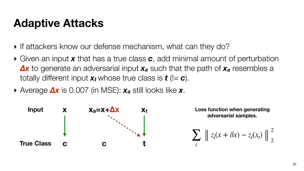
what can they do? ‣ Given an input x that has a true class c, add minimal amount of perturbation Δx to generate an adversarial input xa such that the path of xa resembles a totally different input xt whose true class is t (!= c). ‣ Average Δx is 0.007 (in MSE): xa still looks like x. x c t Input xt True Class xa=x+Δx c ∑ i zi (x + δx) − zi (xt ) 2 2 Loss function when generating adversarial samples.
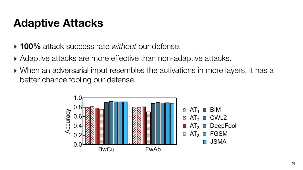
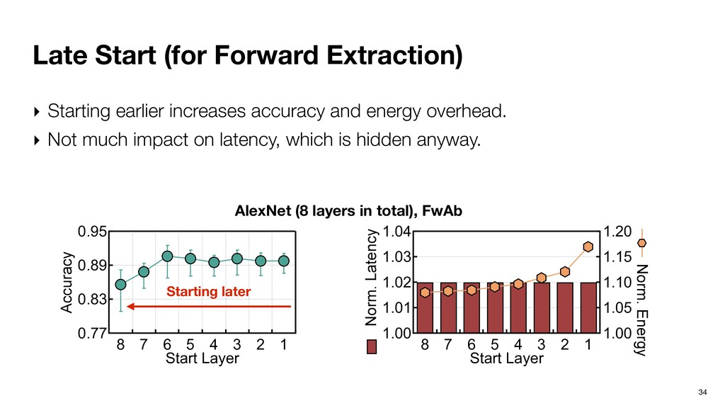
defense. ‣ Adaptive attacks are more effective than non-adaptive attacks. ‣ When an adversarial input resembles the activations in more layers, it has a better chance fooling our defense. 1.0 0.8 0.6 0.4 0.2 0.0 Accuracy BwCu FwAb AT1 BIM AT2 CWL2 AT3 DeepFool AT8 FGSM JSMA
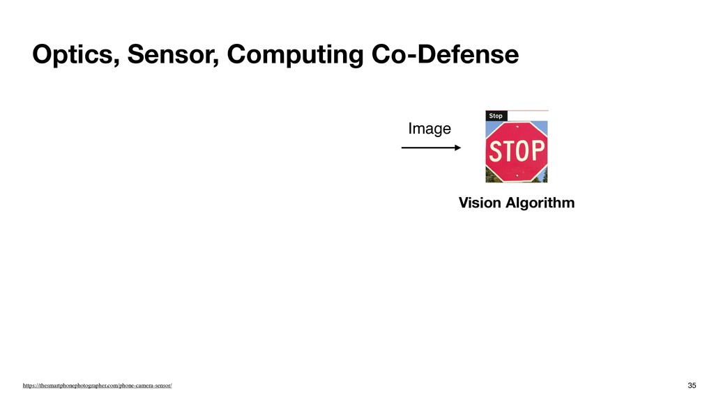
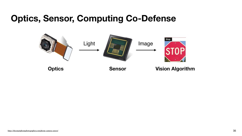
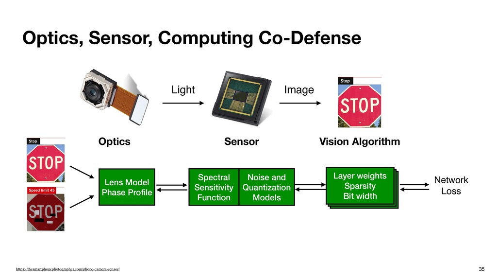
Vision Algorithm How to co-design optics, image sensor, and DNN to improve the system robustness? Lens Model Phase Profile Spectral Sensitivity Function Noise and Quantization Models Layer weights Sparsity Bit width Network Loss
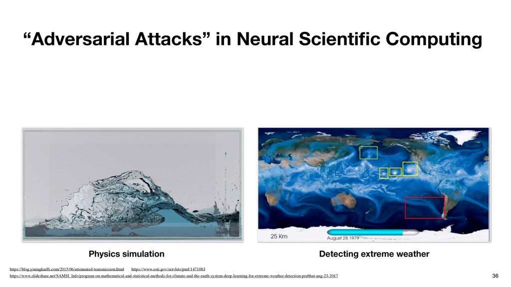
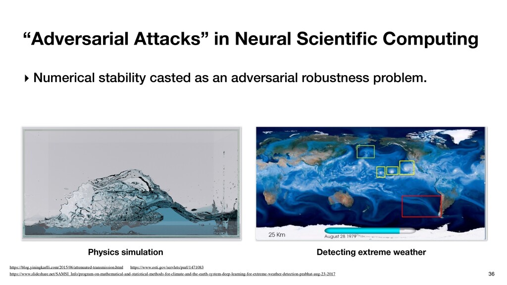
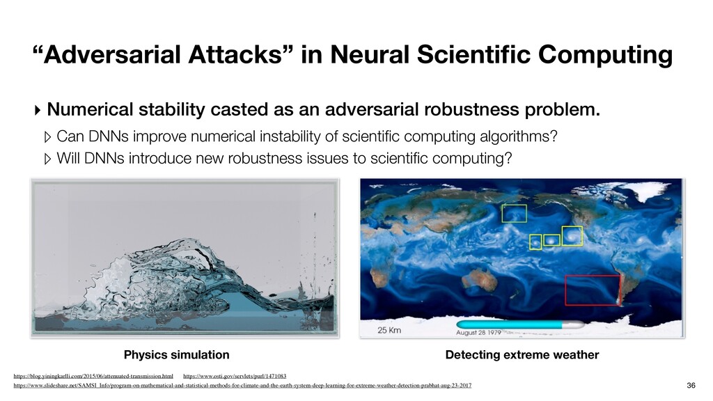
as an adversarial robustness problem. ▹ Can DNNs improve numerical instability of scientific computing algorithms? ▹ Will DNNs introduce new robustness issues to scientific computing? 36 https://blog.yiningkarlli.com/2015/06/attenuated-transmission.html Physics simulation Detecting extreme weather https://www.slideshare.net/SAMSI_Info/program-on-mathematical-and-statistical-methods-for-climate-and-the-earth-system-deep-learning-for-extreme-weather-detection-prabhat-aug-23-2017 https://www.osti.gov/servlets/purl/1471083
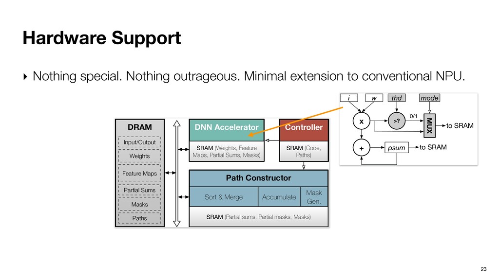
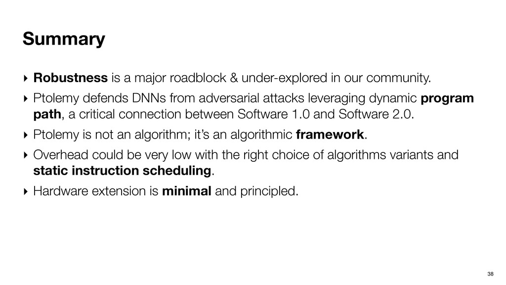
our community. ‣ Ptolemy defends DNNs from adversarial attacks leveraging dynamic program path, a critical connection between Software 1.0 and Software 2.0. ‣ Ptolemy is not an algorithm; it’s an algorithmic framework. ‣ Overhead could be very low with the right choice of algorithms variants and static instruction scheduling. ‣ Hardware extension is minimal and principled. 38
similar to the class path. ‣ Activation paths of adversarial inputs are different from the class path. mple and perturbations from different attacks. The perturbations are enhanced by 100 ti AlexNet on ImageNet Sl = |P(x)l⋂Pl c | P(x)l Activation path for input x at layer l. Class path at layer l. nhanced by 100 times to highlight
more perturbation (Δx) is added, likely because the perturbation is very small — a desirable property. ‣ Ptolemy is not more vulnerable when the attacker simply targets a similar class when generating the attacks. 0.90 0.85 0.80 0.75 0.70 Accuracy 35 30 25 20 15 10 5 0 Distortion/Perturbation (x10-3 MSE) 1.00 0.95 0.90 0.85 0.80 Accuracy 0.30 0.20 0.10 0.00 Path Similarity
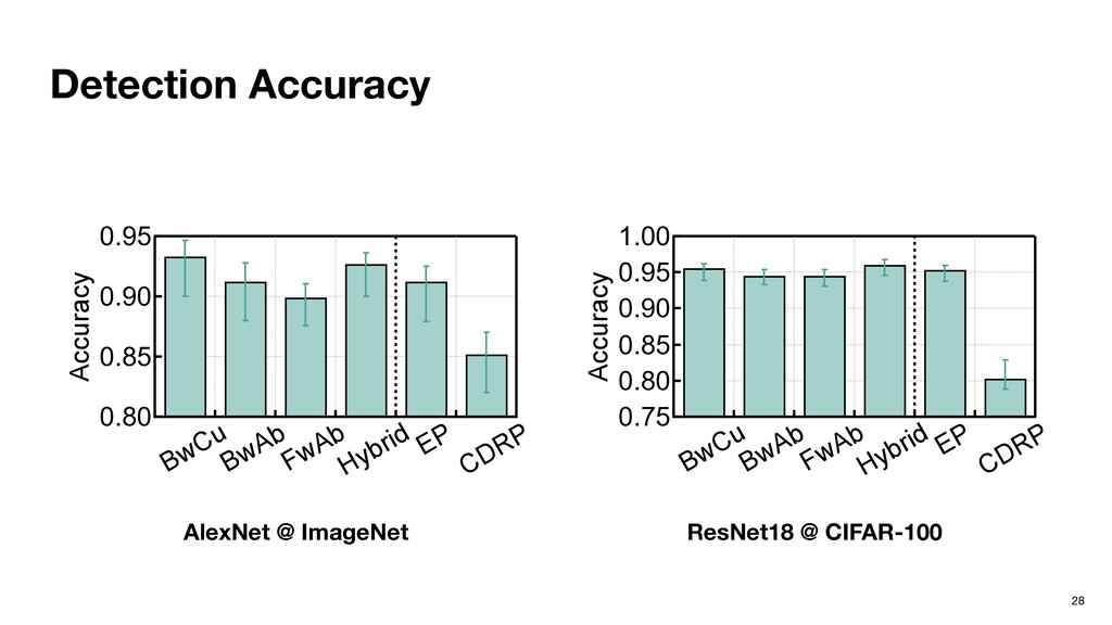
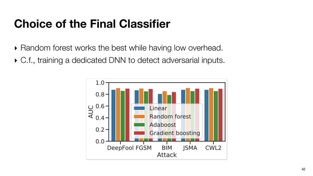
AlexNet on Ima- geNet with weight-based joint simi- larity. Figure 5: Detection accuracy comparison under different (a) Linear model. Figure 7: Impact of attack (a) Linear model. Figure 8: Effective path la 4.1. Detection Accuracy Fig. 5 shows the detecti under different defense mod tacks, we find that random fo linear model performs worst a gap between random forest which indicates that effectiv ‣ Random forest works the best while having low overhead. ‣ C.f., training a dedicated DNN to detect adversarial inputs.