Pangeo NYSDS

Presentation given at the 2019 New York Scientific Data Summit (NYSDS) at Columbia University: https://www.bnl.gov/nysds19/

Transcript

1. Pa n g e o A c o m m u n i t y- d r i v e n e f f o r t f o r 
 B i g D ata g e o s c i e n c e
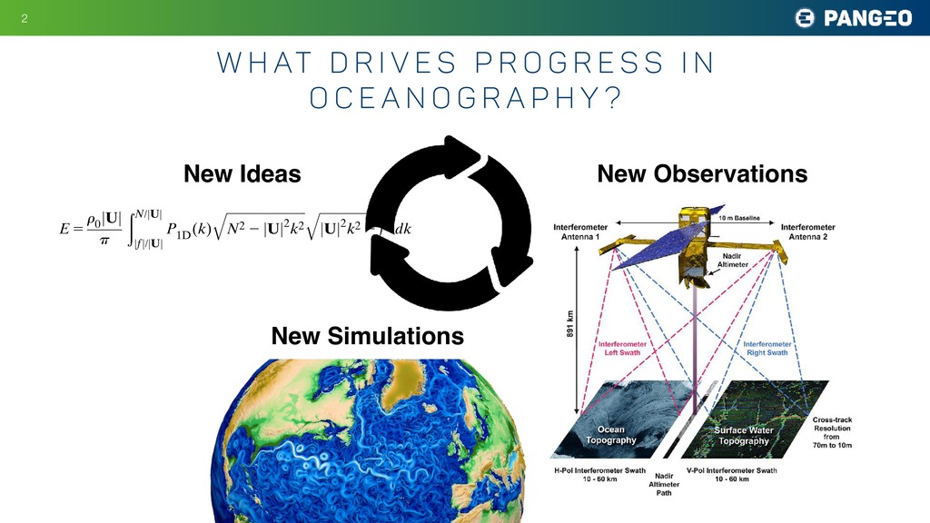
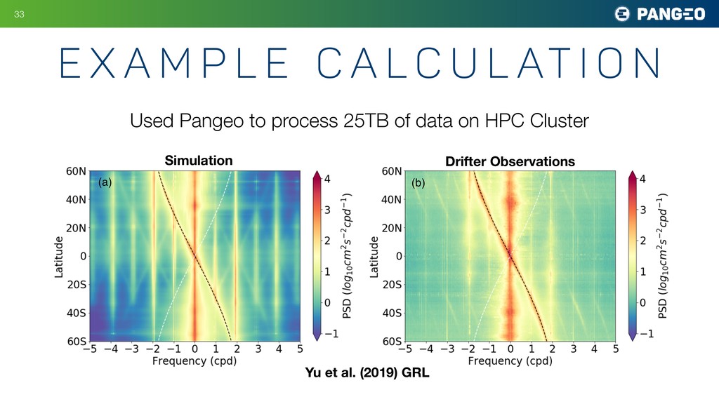
2. !2 W h at D r i v e s P r o g r e s s i n O c e a n o g r a p h y ? New Ideas New Observations New Simulations E 5 r 0 jUj p ðN/jUj jfj/jUj P 1D (k) ffiffiffiffiffiffiffiffiffiffiffiffiffiffiffiffiffiffiffiffiffiffiffiffiffi ffi N2 2 jUj2k2 q ffiffiffiffiffiffiffiffiffiffiffiffiffiffiffiffiffiffiffiffiffiffiffiffi jUj2k2 2 f2 q dk, (3) where k 5 (k, l) is now the wavenumber in the reference frame along and across the mean flow U and P 1D (k) 5 1 2p ð1‘ 2‘ jkj jkj P 2D (k, l) dl (4) is the effective one-dimensional (1D) topographic spectrum. Hence, the wave radiation from 2D topogra- phy reduces to an equivalent problem of wave radiation from 1D topography with the effective spectrum given by P1D (k). The effective 1D spectrum captures the effects of 2D c. Bottom topography Simulations are configured with multiscale topogra- phy characterized by small-scale abyssal hills a few ki- lometers wide based on multibeam observations from Drake Passage. The topographic spectrum associated with abyssal hills is well described by an anisotropic parametric representation proposed by Goff and Jordan (1988): P 2D (k, l) 5 2pH2(m 2 2) k 0 l 0 1 1 k2 k2 0 1 l2 l2 0 !2m/2 , (5) where k0 and l0 set the wavenumbers of the large hills, m is the high-wavenumber spectral slope, related to the pa- FIG. 3. Averaged profiles of (left) stratification (s21) and (right) flow speed (m s21) in the bottom 2 km from observations (gray), initial condition in the simulations (black), and final state in 2D (blue) and 3D (red) simulations.
3. !3 MITgcm LLC4320 Simulation Grid resolution:
 1 - 2 km Single 3D scalar field:
 80 GB Output frequency: 1 hour Simulation Length: 1 year Output data volume: 2 PB Credit: NASA JPL / Dimitris Menemenlis
4. C o m p u t e r A r c h i t e c t u r e !4 CC by 4.0 by Karl upp CC by 4.0 by Karl Rupp via Willi Rath (GEOMAR)
5. C o m p u t e r A r c h i t e c t u r e !5 Adapted from image by Karl upp CC by 4.0 by Karl Rupp via Willi Rath (GEOMAR)
6. !6 C o m p u t e r a r c h i t e c t u r e : 
 S i m u l at i o n NASA Pleaides Supercomputer
7. !7 C o m p u t e r a r c h i t e c t u r e : 
 A n a ly s i s a n d V i s u a l i z at i o n
8. Adapted from image by Karl upp C o m p u t e r A r c h i t e c t u r e !8 CC by 4.0 by Karl Rupp via Willi Rath (GEOMAR)
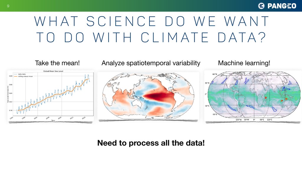
9. !9 W h at S c i e n c e d o w e w a n t t o d o w i t h c l i m at e d ata? Take the mean! Analyze spatiotemporal variability Machine learning! Need to process all the data!
10. Pa n g e o C h a l l e n g e !10 How can we develop flexible analysis tools that meet our community’s diverse needs and scale to Petabyte-sized datasets?
11. • Open Community • Open Source Software • Open Source Infrastructure !11 W h at i s Pa n g e o ? “A community platform for Big Data geoscience”
12. !12 Pa n g e o C o m m u n i t y http://pangeo.io
13. !13 Pa n g e o F u n d i n g http://pangeo.io
14. Pa n g e o S o f t w a r e !14
15. !15 source: stackoverflow.com S c i e n t i f i c P y t h o n f o r D ata S c i e n c e
16. aospy S c i e n t i f i c P y t h o n f o r C l i m at e !16 SciPy Credit: Stephan Hoyer, Jake Vanderplas (SciPy 2015)
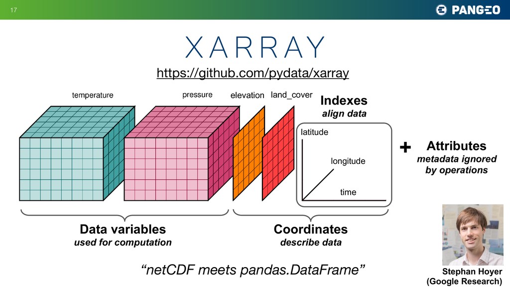
17. X a r r ay !17 time longitude latitude elevation Data variables used for computation Coordinates describe data Indexes align data Attributes metadata ignored by operations + land_cover “netCDF meets pandas.DataFrame” Stephan Hoyer
 (Google Research) https://github.com/pydata/xarray
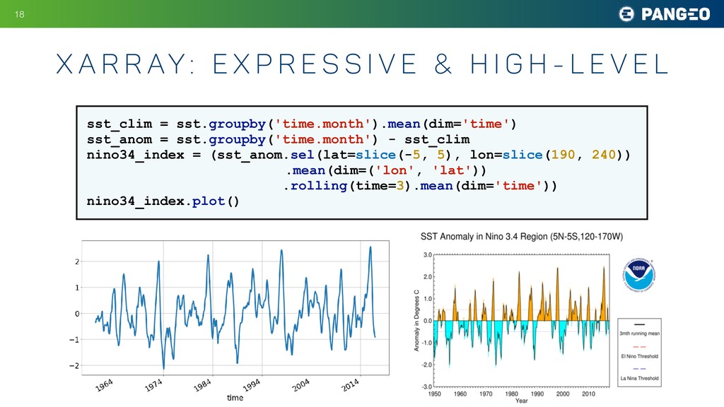
18. x a r r ay : E x p r e s s i v e & h i g h - l e v e l !18 sst_clim = sst.groupby('time.month').mean(dim='time') sst_anom = sst.groupby('time.month') - sst_clim nino34_index = (sst_anom.sel(lat=slice(-5, 5), lon=slice(190, 240)) .mean(dim=('lon', 'lat')) .rolling(time=3).mean(dim='time')) nino34_index.plot()
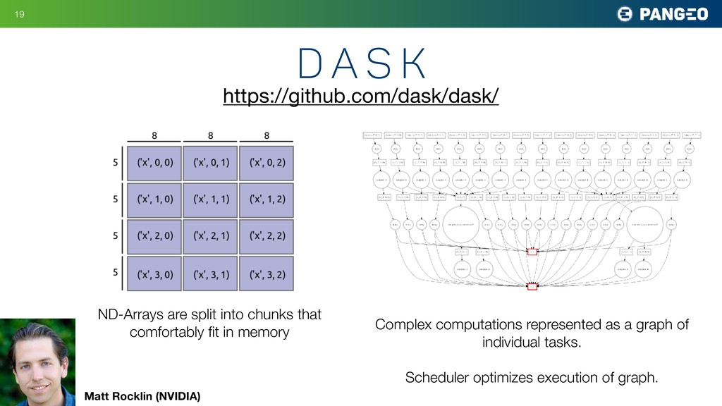
19. d a s k !19 Complex computations represented as a graph of individual tasks. 
 Scheduler optimizes execution of graph. https://github.com/dask/dask/ ND-Arrays are split into chunks that comfortably fit in memory Matt Rocklin (NVIDIA)
20. J u p y t e r !20 “Project Jupyter exists to develop open-source software, open-standards, and services for interactive computing across dozens of programming languages.”
21. Pa n g e o I n f r a s t r u c t u r e !21
22. F i l e - b a s e d A p p r o a c h !22 a) file-based approach step 1 : dow nload step 2: analyze ` file file file b) database approach file file file local disk files Data provider’s responsibilities End user’s responsibilities
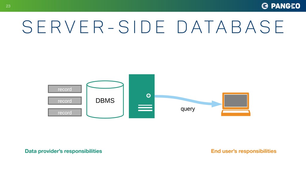
23. S e r v e r - S i d e D ata b a s e !23 ` file file file b) database approach record record record DBMS file file file local disk query c) cloud approach files Data provider’s responsibilities End user’s responsibilities
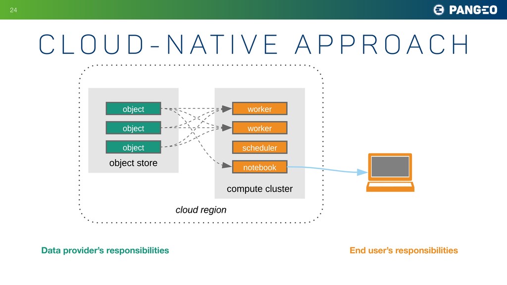
24. C l o u d - N at i v e A p p r o a c h !24 object store record query c) cloud approach object object object cloud region compute cluster worker worker scheduler notebook Data provider’s responsibilities End user’s responsibilities
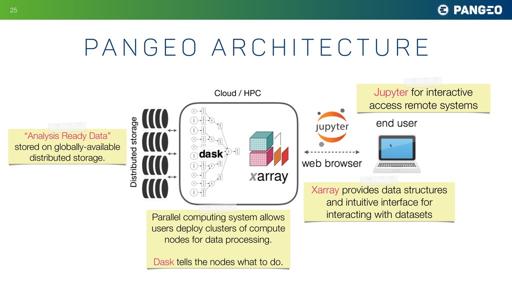
25. !25 Pa n g e o A r c h i t e c t u r e Jupyter for interactive access remote systems Cloud / HPC Xarray provides data structures and intuitive interface for interacting with datasets Parallel computing system allows users deploy clusters of compute nodes for data processing. Dask tells the nodes what to do. Distributed storage “Analysis Ready Data”
 stored on globally-available distributed storage.
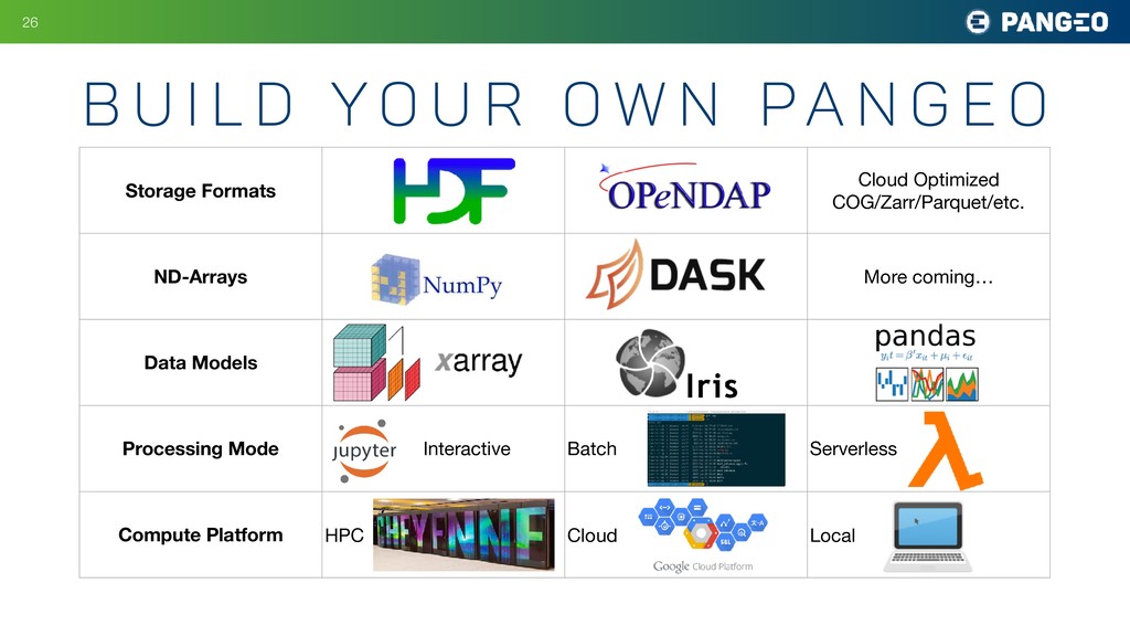
26. !26 B u i l d y o u r o w n pa n g e o Storage Formats Cloud Optimized COG/Zarr/Parquet/etc. ND-Arrays More coming… Data Models Processing Mode Interactive Batch Serverless Compute Platform HPC Cloud Local
27. !27 Pa n g e o D e p l o y m e n t s NASA Pleiades pa n g e o . p y d ata . o r g NCAR Cheyenne Over 1000 unique users since March http://pangeo.io/deployments.html
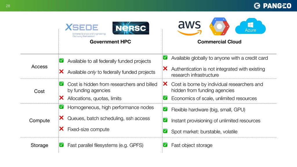
28. !28 Government HPC Commercial Cloud Access ✅ Available to all federally funded projects ❌ Available only to federally funded projects ✅ Available globally to anyone with a credit card ❌ Authentication is not integrated with existing research infrastructure Cost ✅ Cost is hidden from researchers and billed by funding agencies ❌ Allocations, quotas, limits ❌ Cost is borne by individual researchers and hidden from funding agencies ✅ Economics of scale, unlimited resources Compute ✅ Homogeneous, high performance nodes ❌ Queues, batch scheduling, ssh access ❌ Fixed-size compute ✅ Flexible hardware (big, small, GPU) ✅ Instant provisioning of unlimited resources ✅ Spot market: burstable, volatile Storage ✅ Fast parallel filesystems (e.g. GPFS) ✅ Fast object storage
29. • https://github.com/pangeo- data/pangeo-cloud-federation • Cloud-based clusters managed with helm /kubernetes • Deployment is completely automated via GitHub / circleci • Resources scale elastically with demand !29 C o n t i n u o u s D e p l o y m e n t
30. • https://pangeo-data.github.io/ pangeo-datastore/ • Datasets stored in zarr format (cloud-native HDF-replacement) • Cataloged using intake • Automated testing of datasets !30 C l o u d D ata C ata l o g
31. C l o u d C o s t s !31
32. D E M O !32 https://tinyurl.com/pangeo-ocean
33. E x a m p l e C a l c u l at i o n !33 (a) (b) (c) Yu et al. (2019) GRL Used Pangeo to process 25TB of data on HPC Cluster Simulation Drifter Observations
34. C M I P 6 H a c k at h o n !34 https://cmip6hack.github.io
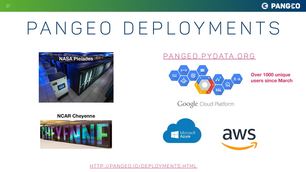
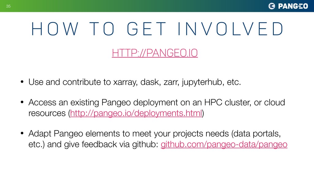
35. • Use and contribute to xarray, dask, zarr, jupyterhub, etc. • Access an existing Pangeo deployment on an HPC cluster, or cloud resources (http://pangeo.io/deployments.html) • Adapt Pangeo elements to meet your projects needs (data portals, etc.) and give feedback via github: github.com/pangeo-data/pangeo !35 H o w t o g e t i n v o lv e d http://pangeo.io
36. !36