Statistical Rethinking 2022 Lecture 07

Course description: https://github.com/rmcelreath/stat_rethinking_2022

Transcript

1. Statistical Rethinking 07: Fitting Over and Under 2022
2. Mikołaj Kopernik (1473–1543)
3. Copernican Model
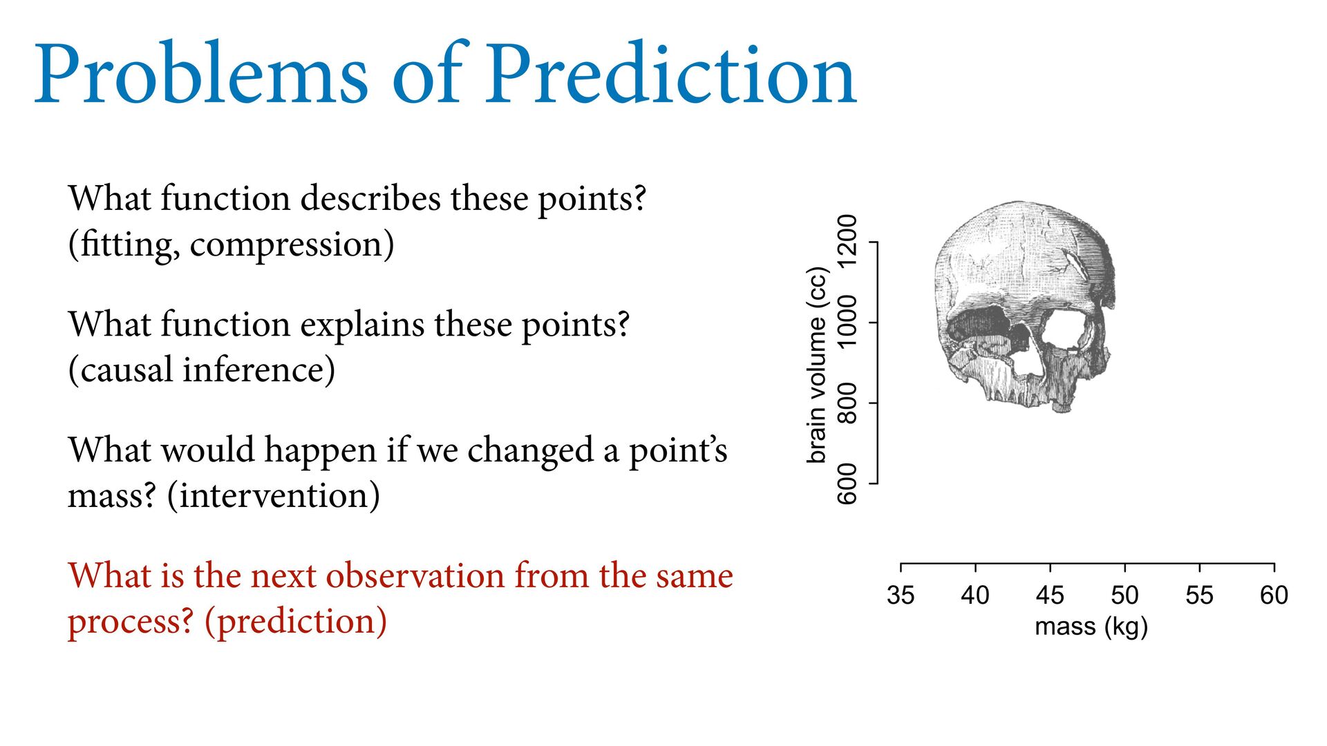
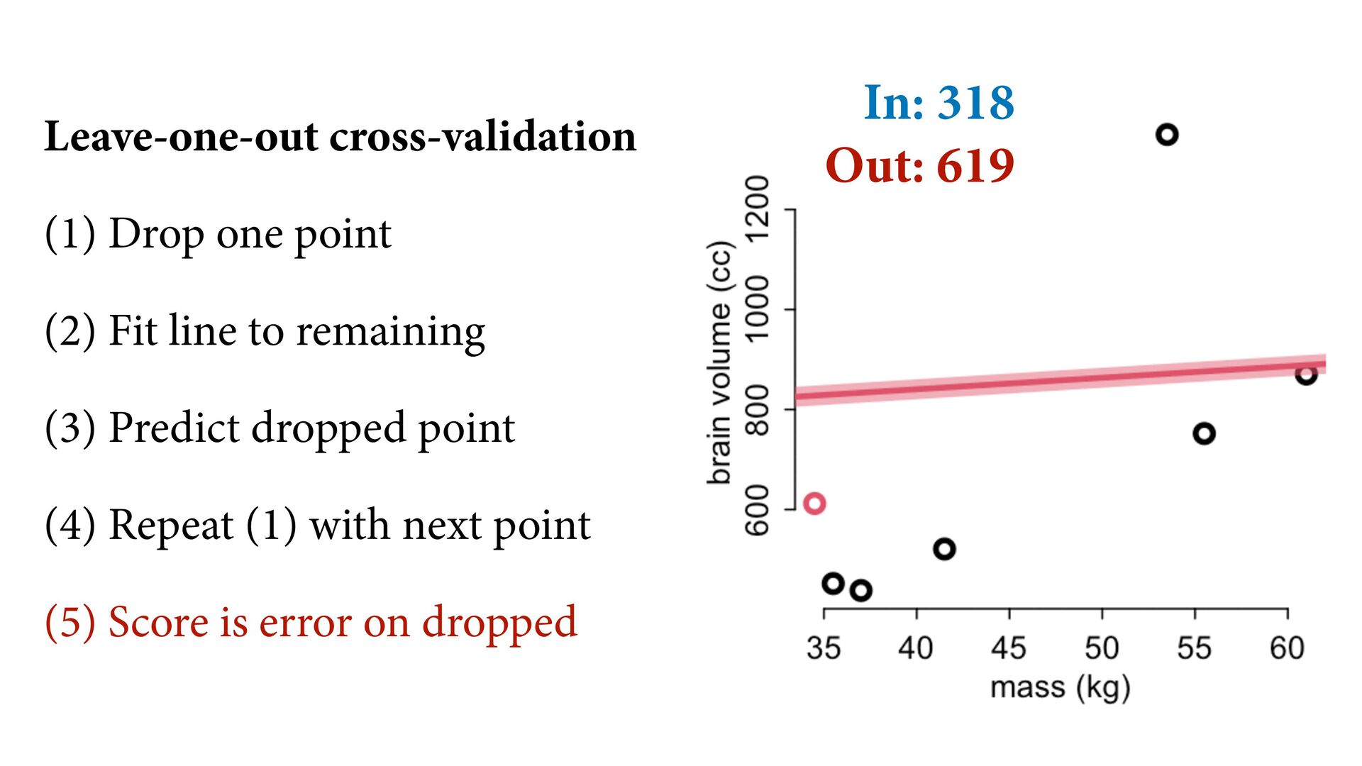
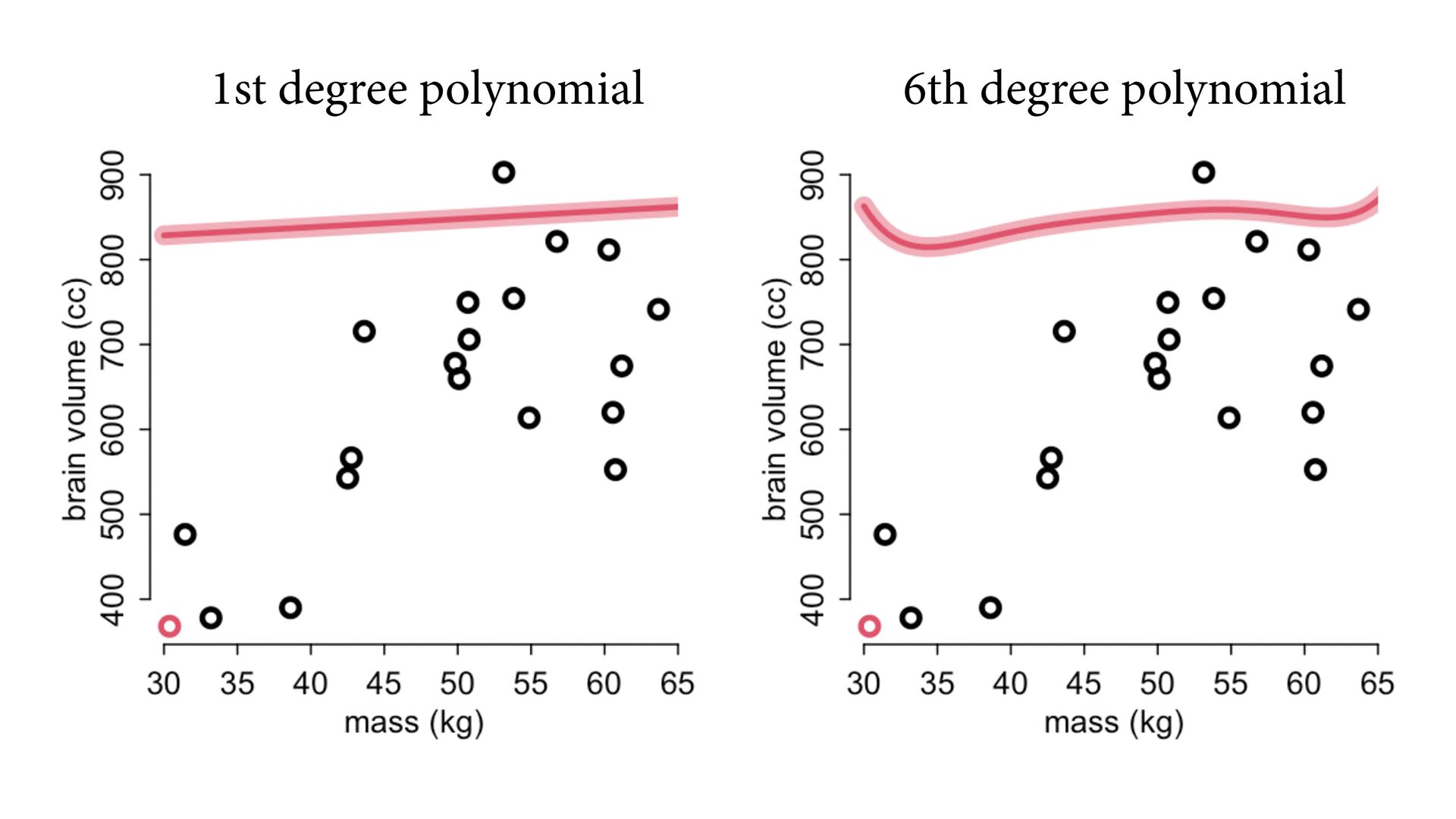
4. Problems of Prediction What function describes these points? (fitting, compression) What function explains these points? (causal inference) What would happen if we changed a point’s mass? (intervention) What is the next observation from the same process? (prediction) 35 40 45 50 55 60 600 800 1000 1200 mass (kg) brain volume (cc)
5. Leave-one-out cross-validation (1) Drop one point (2) Fit line to remaining (3) Predict dropped point (4) Repeat (1) with next point (5) Score is error on dropped
6. Leave-one-out cross-validation (1) Drop one point (2) Fit line to remaining (3) Predict dropped point (4) Repeat (1) with next point (5) Score is error on dropped
7. Leave-one-out cross-validation (1) Drop one point (2) Fit line to remaining (3) Predict dropped point (4) Repeat (1) with next point (5) Score is error on dropped
8. Leave-one-out cross-validation (1) Drop one point (2) Fit line to remaining (3) Predict dropped point (4) Repeat (1) with next point (5) Score is error on dropped
9. Leave-one-out cross-validation (1) Drop one point (2) Fit line to remaining (3) Predict dropped point (4) Repeat (1) with next point (5) Score is error on dropped In: 318 Out: 619
10. Bayesian Cross-Validation We use the entire posterior, not just a point prediction Cross-validation score is: MJNJU UIFPSFN UP QSPWJEF B NFBTVSF PG UIF TUBOEBSE FSSPS TĽŀĶŀ = / WBS(QTJT J) NCFS PG PCTFSWBUJPOT BOE QTJT J JT UIF 14*4 FTUJNBUF GPS PCTFSWBUJPO J *G UIJT F TFOTF CF TVSF UP MPPL BU UIF DPEF CPY BU UIF FOE PG UIJT TFDUJPO QBHF   FUPTNPPUIFE DSPTTWBMJEBUJPO $SPTTWBMJEBUJPO FTUJNBUFT UIF PVUPGTBNQMF ĿIJıĶİŁĶŃIJıIJĻŀĶŁņ MQQE QBHF   *G ZPV IBWF / PCTFSWBUJPOT BOE ĕU UIF QQJOH B TJOHMF PCTFSWBUJPO ZJ FBDI UJNF UIFO UIF PVUPGTBNQMF MQQE JT UIF TVN BDZ GPS FBDI PNJUUFE ZJ  MQQE $7 = / J=  4 4 T= MPH 1S(ZJ|θ−J,T) NQMFT GSPN B .BSLPW DIBJO BOE θ−J,T JT UIF TUI TBNQMF GSPN UIF QPTUFSJPS EJTUSJ S PCTFSWBUJPOT PNJUUJOH ZJ  NQMJOH SFQMBDFT UIF DPNQVUBUJPO PG / QPTUFSJPS EJTUSJCVUJPOT CZ VTJOH BO FTUJNBUF -5 -4 -3 -2 -1 0 0.0 0.5 1.0 1.5 log posterior prob of observation Density
11. Bayesian Cross-Validation FSF / JT UIF OVNCFS PG PCTFSWBUJPOT BOE QTJT J JT UIF 14*4 FTUJNBUF GPS PCTFSWBUJPO J *G TOU RVJUF NBLF TFOTF CF TVSF UP MPPL BU UIF DPEF CPY BU UIF FOE PG UIJT TFDUJPO QBHF  FSUIJOLJOH 1BSFUPTNPPUIFE DSPTTWBMJEBUJPO $SPTTWBMJEBUJPO FTUJNBUFT UIF PVUPGTBN ĴĽļĶĻŁńĶŀIJĽĿIJıĶİŁĶŃIJıIJĻŀĶŁņ MQQE QBHF   *G ZPV IBWF / PCTFSWBUJPOT BOE ĕU EFM / UJNFT ESPQQJOH B TJOHMF PCTFSWBUJPO ZJ FBDI UJNF UIFO UIF PVUPGTBNQMF MQQE JT UIF T IF BWFSBHF BDDVSBDZ GPS FBDI PNJUUFE ZJ  MQQE $7 = / J=  4 4 T= MPH 1S(ZJ|θ−J,T) SF T JOEFYFT TBNQMFT GSPN B .BSLPW DIBJO BOE θ−J,T JT UIF TUI TBNQMF GSPN UIF QPTUFSJPS EJ PO DPNQVUFE GPS PCTFSWBUJPOT PNJUUJOH ZJ  *NQPSUBODF TBNQMJOH SFQMBDFT UIF DPNQVUBUJPO PG / QPTUFSJPS EJTUSJCVUJPOT CZ VTJOH BO FTUJN IF JNQPSUBODF PG FBDI J UP UIF QPTUFSJPS EJTUSJCVUJPO 8F ESBX TBNQMFT GSPN UIF GVMM QPTUFSJPS VUJPO Q(θ|Z) CVU XF XBOU TBNQMFT GSPN UIF SFEVDFE MFBWFPOFPVU QPTUFSJPS EJTUSJCVUJPO Q(θ|Z XF SFXFJHIU FBDI TBNQMF T CZ UIF JOWFSTF PG UIF QSPCBCJMJUZ PG UIF PNJUUFE PCTFSWBUJPO  log pointwise predictive density Pages 210 and 218 N data points S samples from posterior log probability of each point i, computed with posterior that omits point i average log probability for point i
12. In: 318 Out: 619 In: 289 Out: 865 [1] [2]
13. 318 619 289 865 In: 201 Out: 12,538 [3] [1] [2]
14. 201 12,538 120 25,530 7 293,840 318 619 289 865 [1] [2] [3] [4] [5]
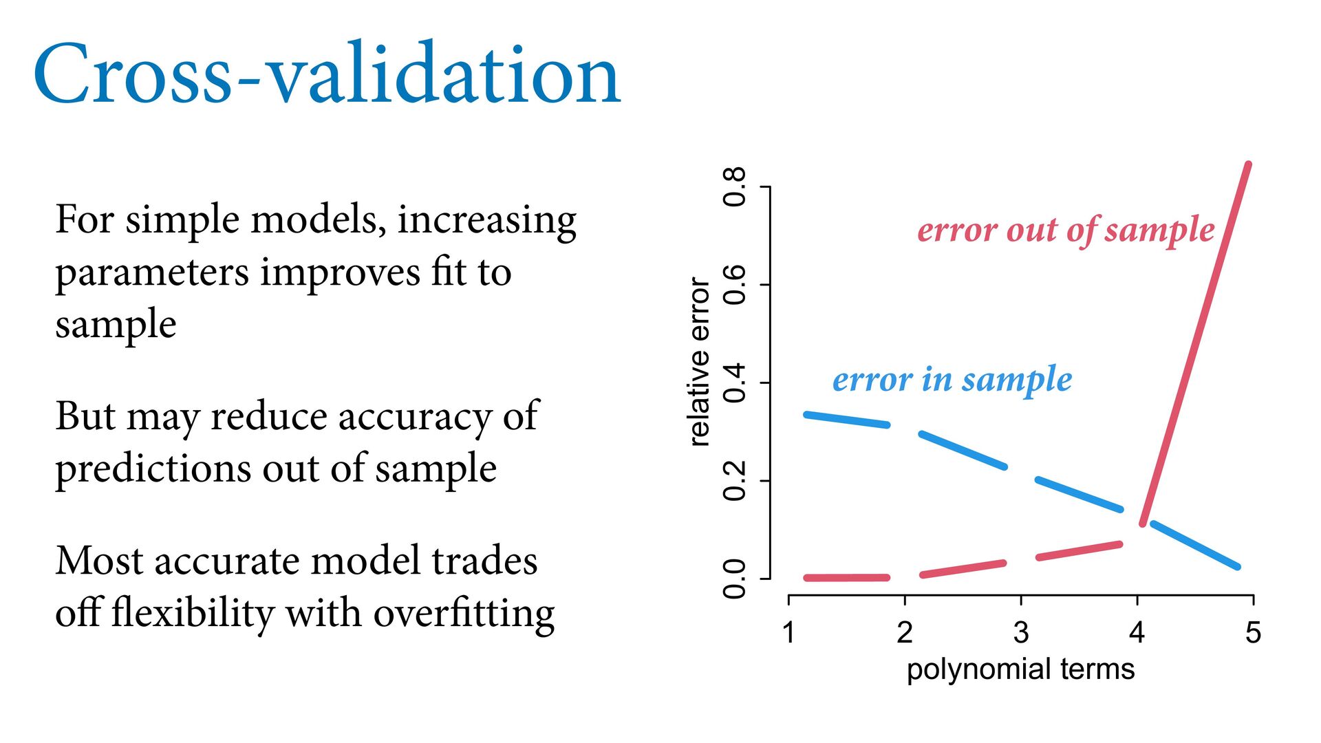
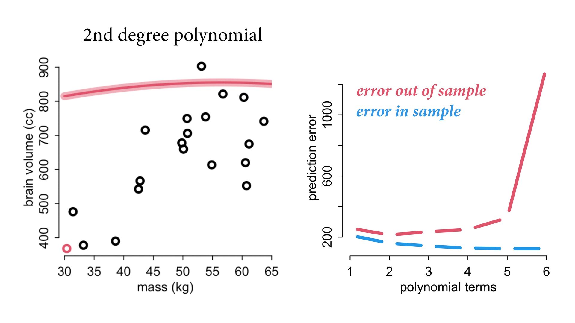
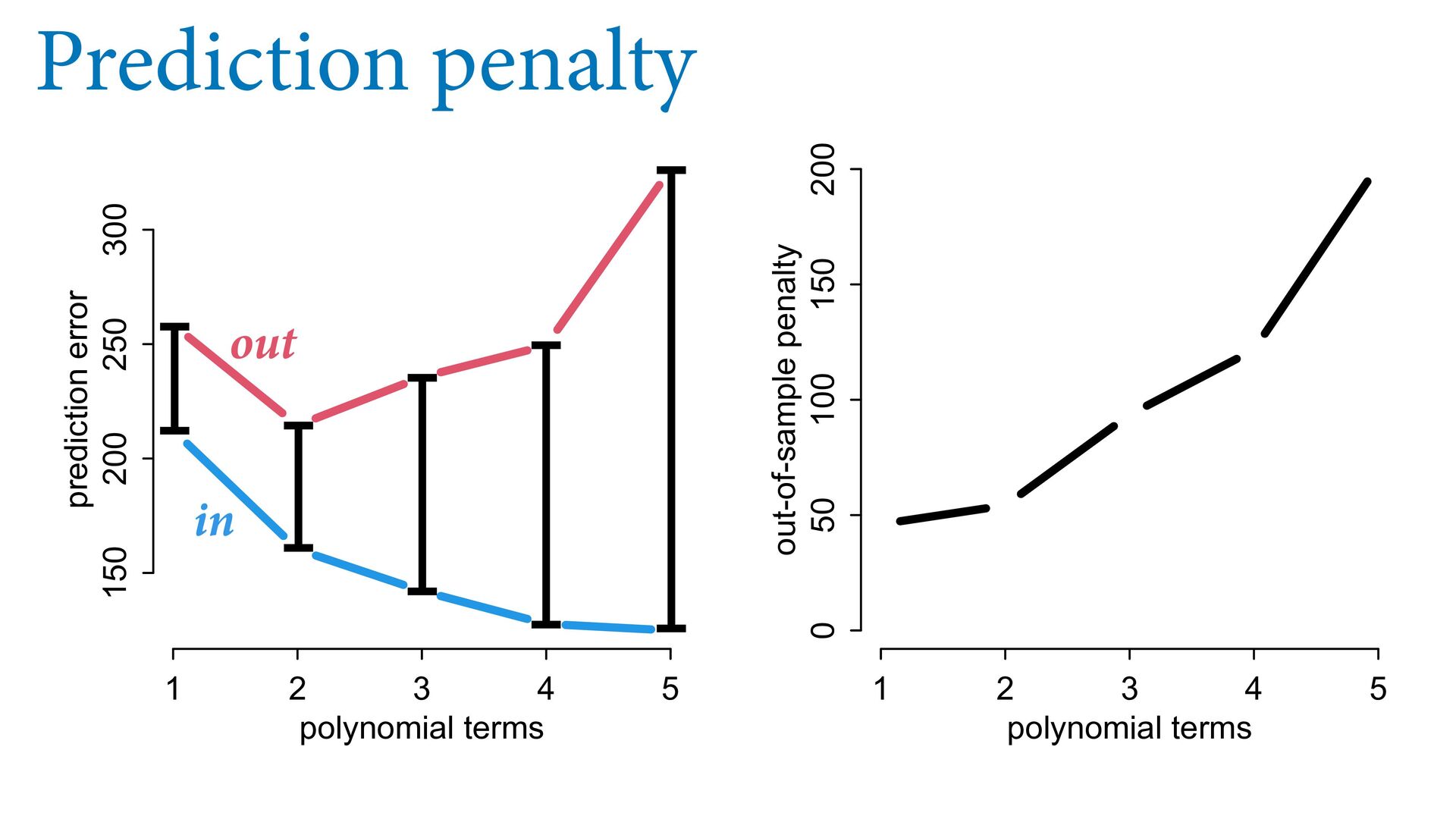
15. Cross-validation For simple models, increasing parameters improves fit to sample But may reduce accuracy of predictions out of sample Most accurate model trades off flexibility with overfitting 1 2 3 4 5 0.0 0.2 0.4 0.6 0.8 polynomial terms relative error error in sample error out of sample
16. 1st degree polynomial 6th degree polynomial
17. 2nd degree polynomial error in sample error out of sample 1 2 3 4 5 6 200 600 1000 polynomial terms prediction error
18. 2nd degree polynomial error in sample error out of sample 1 2 3 4 5 150 200 250 300 polynomial terms prediction error
19. Regularization Overfitting depends upon the priors Skeptical priors have tighter variance, reduce flexibility Regularization: Function finds regular features of process Good priors are often tighter than you think!
20. 1 2 3 4 5 150 200 250 300 polynomial terms prediction error in out β j ∼ Normal(0,10) μ i = α + m ∑ j= 1 β j xj i
21. 1 2 3 4 5 150 200 250 300 polynomial terms prediction error in out β j ∼ Normal(0,10) β j ∼ Normal(0,10) β j ∼ Normal(0,1) β j ∼ Normal(0,1)
22. 1 2 3 4 5 150 200 250 300 polynomial terms prediction error in out β j ∼ Normal(0,10) β j ∼ Normal(0,10) β j ∼ Normal(0,1) β j ∼ Normal(0,1) β j ∼ Normal(0,0.5) β j ∼ Normal(0,0.5)
23. in out 1 2 3 4 5 150 200 250 300 350 400 polynomial terms prediction error β j ∼ Normal(0,0.1)
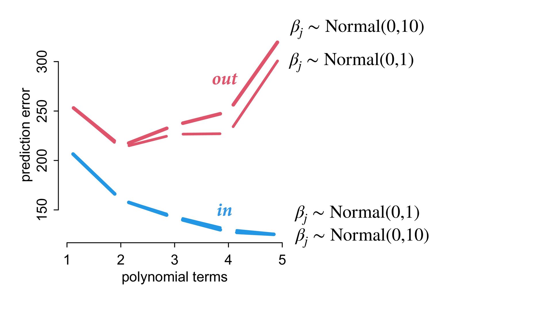
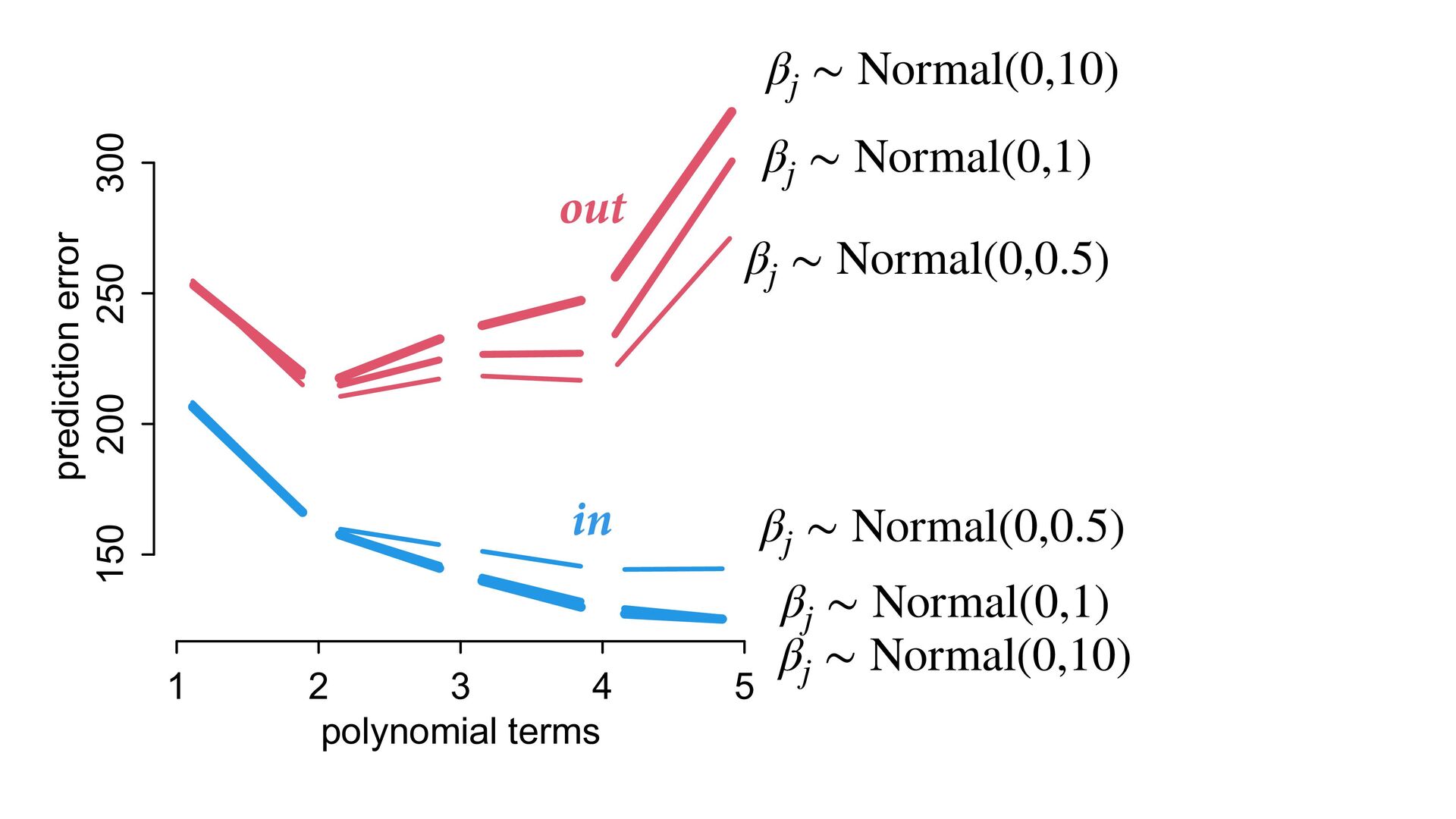
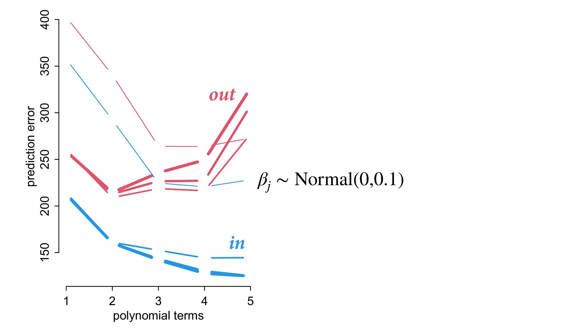
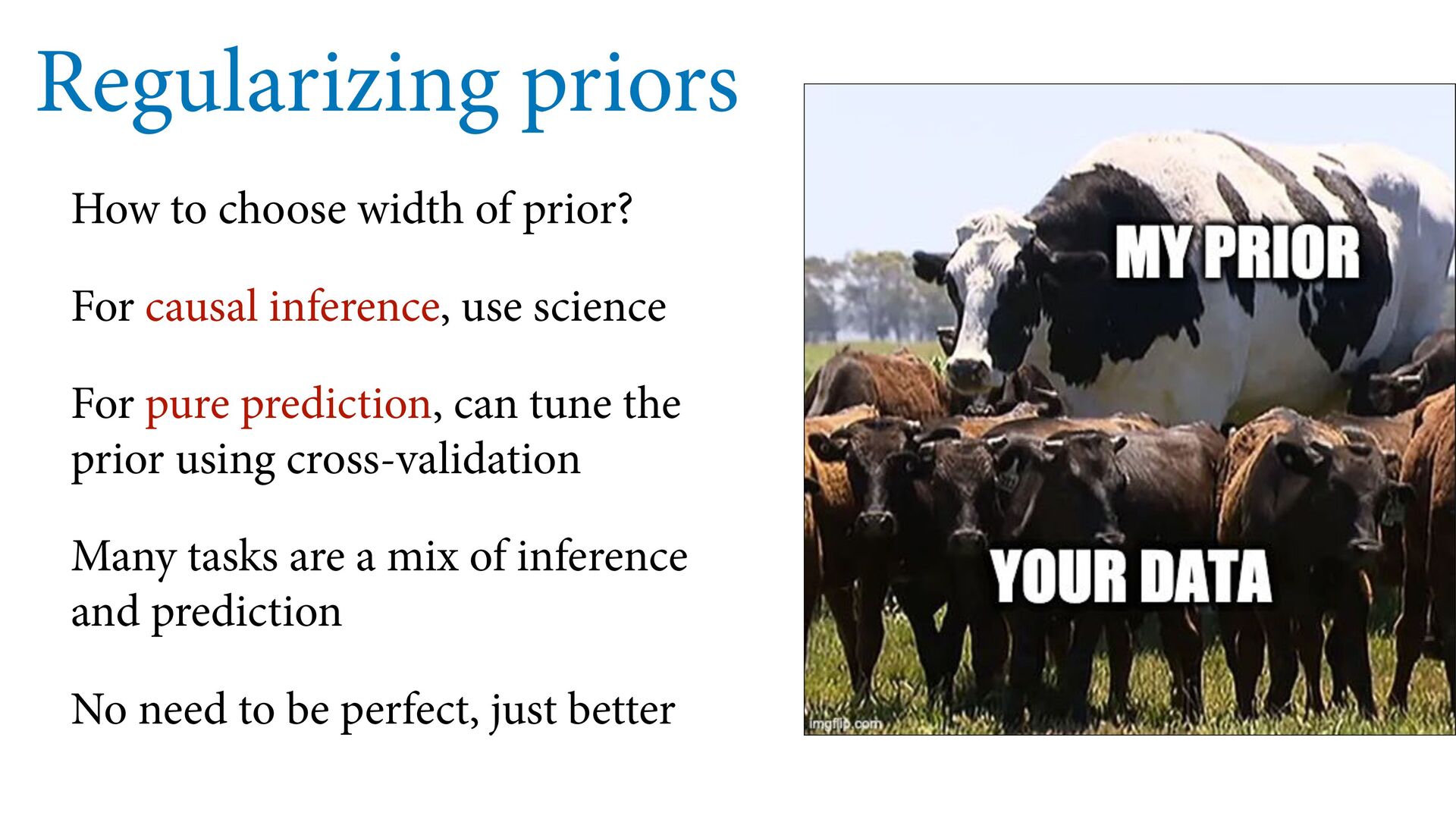
24. Regularizing priors How to choose width of prior? For causal inference, use science For pure prediction, can tune the prior using cross-validation Many tasks are a mix of inference and prediction No need to be perfect, just better
25. PAUSE
26. Prediction penalty 1 2 3 4 5 150 200 250 300 polynomial terms prediction error 1 2 3 4 5 0 50 100 150 200 polynomial terms out-of-sample penalty in out
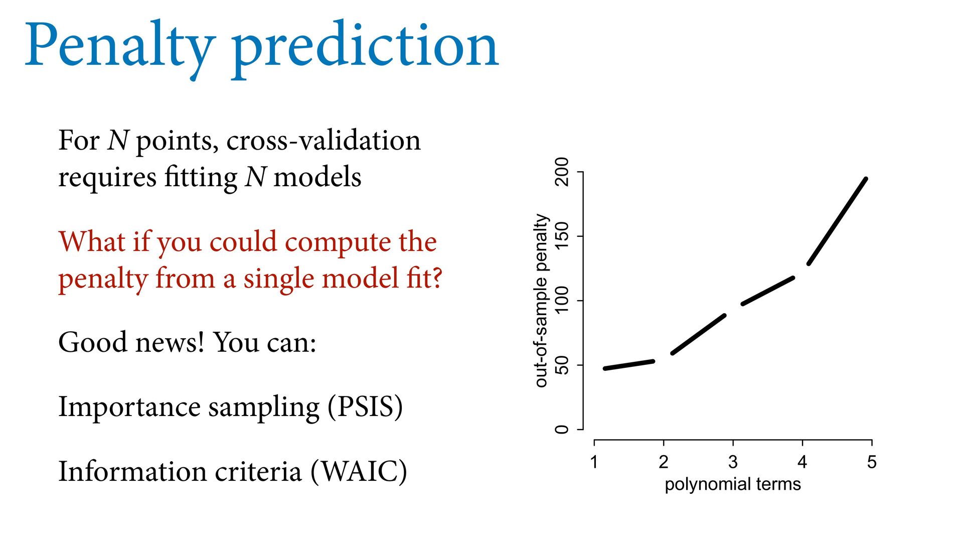
27. Penalty prediction For N points, cross-validation requires fitting N models What if you could compute the penalty from a single model fit? Good news! You can: Importance sampling (PSIS) Information criteria (WAIC) 1 2 3 4 5 0 50 100 150 200 polynomial terms out-of-sample penalty
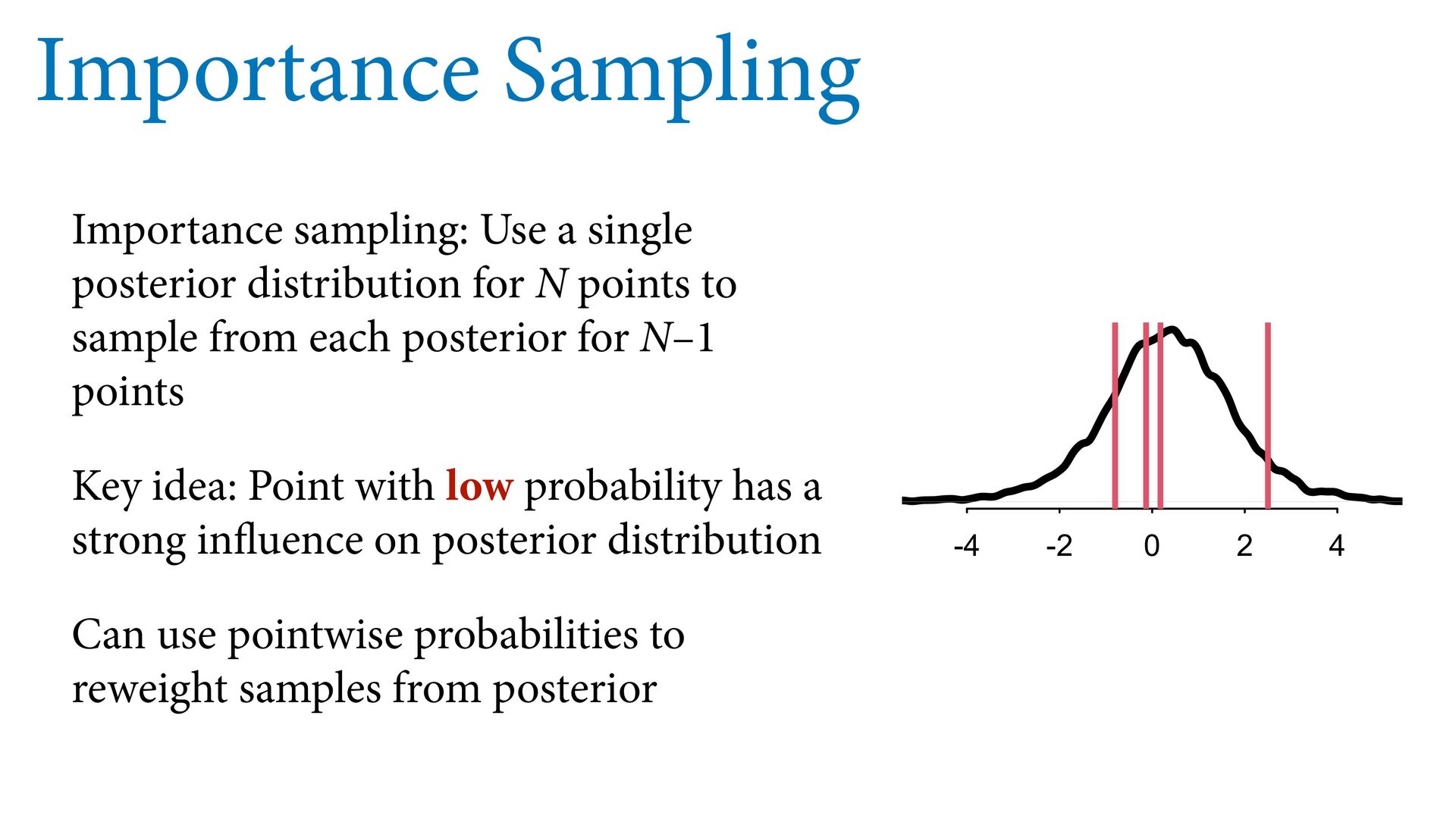
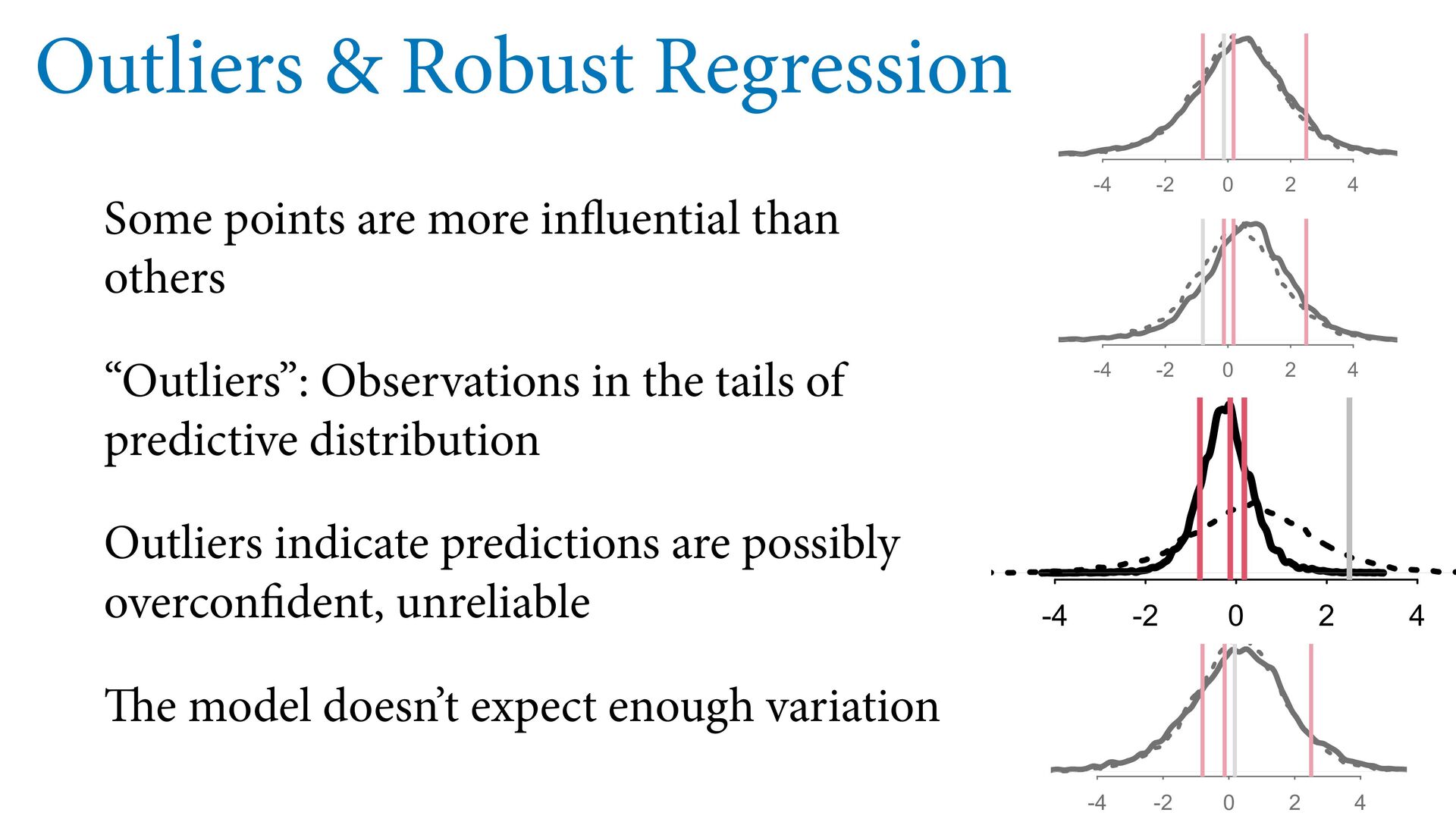
28. Importance Sampling Importance sampling: Use a single posterior distribution for N points to sample from each posterior for N–1 points Key idea: Point with low probability has a strong influence on posterior distribution Can use pointwise probabilities to reweight samples from posterior -4 -2 0 2 4
29. -4 -2 0 2 4 observations posterior
30. -4 -2 0 2 4 -4 -2 0 2 4 -4 -2 0 2 4 -4 -2 0 2 4 -4 -2 0 2 4
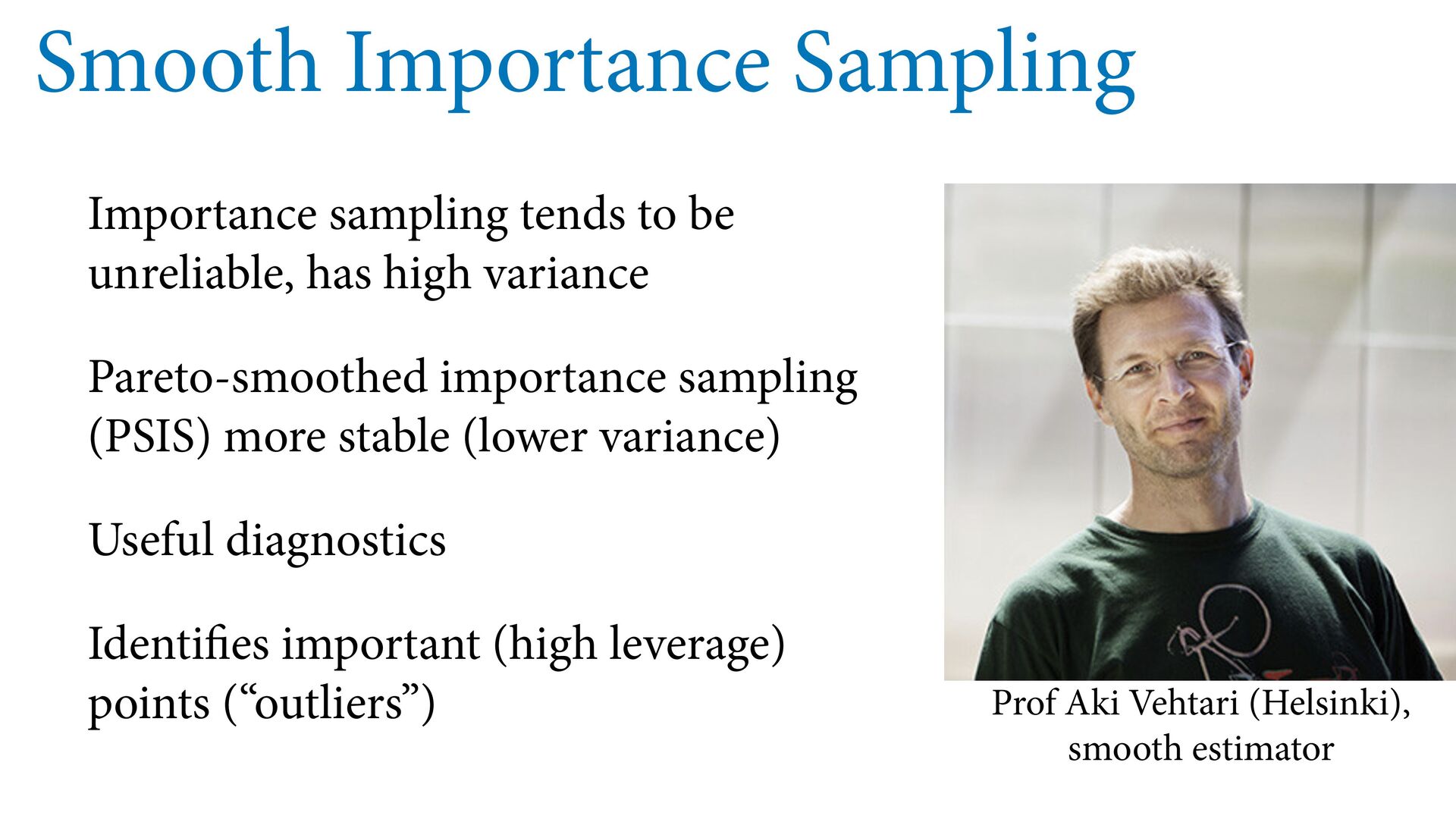
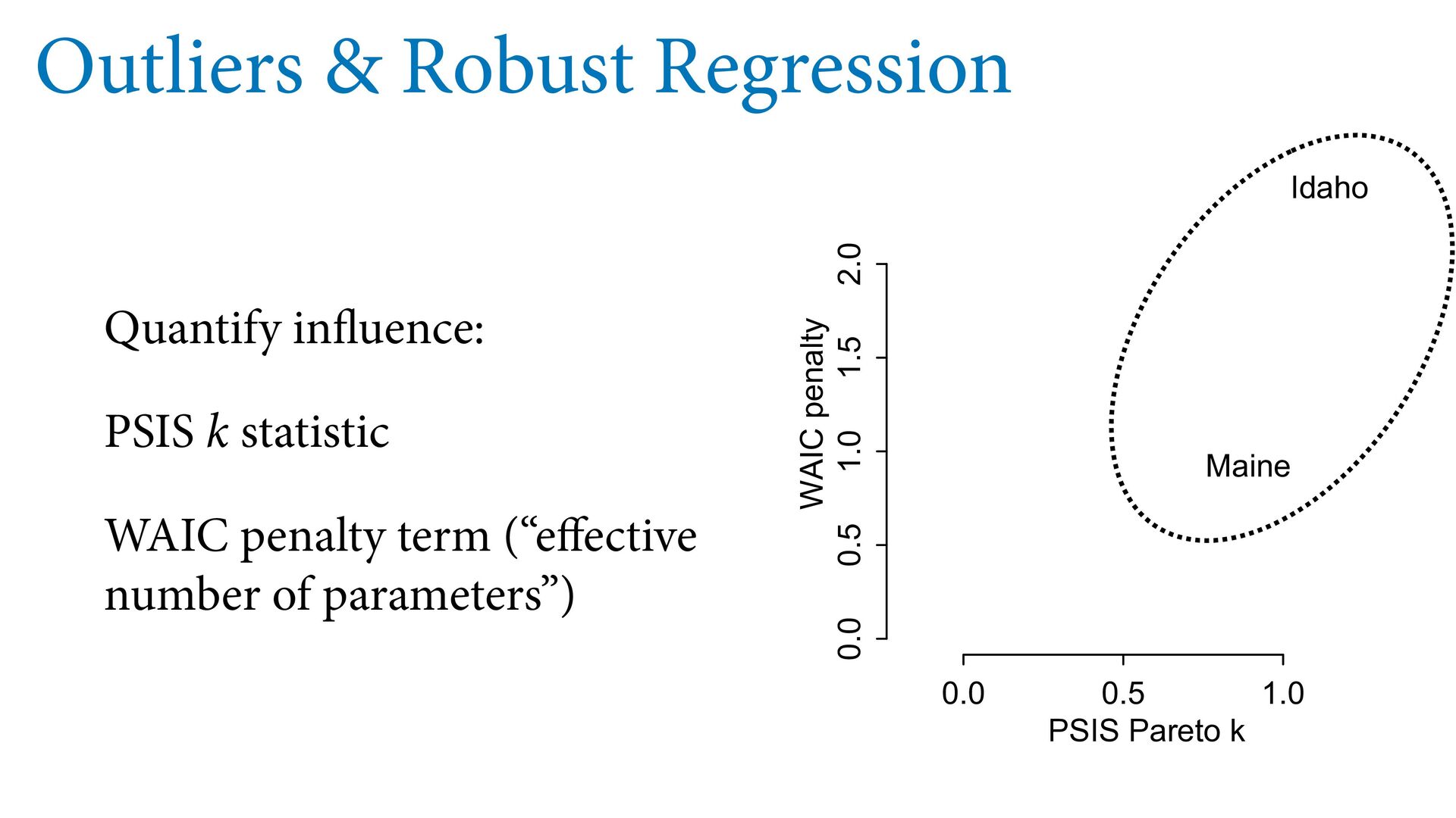
31. Smooth Importance Sampling Prof Aki Vehtari (Helsinki), smooth estimator Importance sampling tends to be unreliable, has high variance Pareto-smoothed importance sampling (PSIS) more stable (lower variance) Useful diagnostics Identifies important (high leverage) points (“outliers”)
32. Akaike information criterion Estimate information-theoretic measure of predictive accuracy 
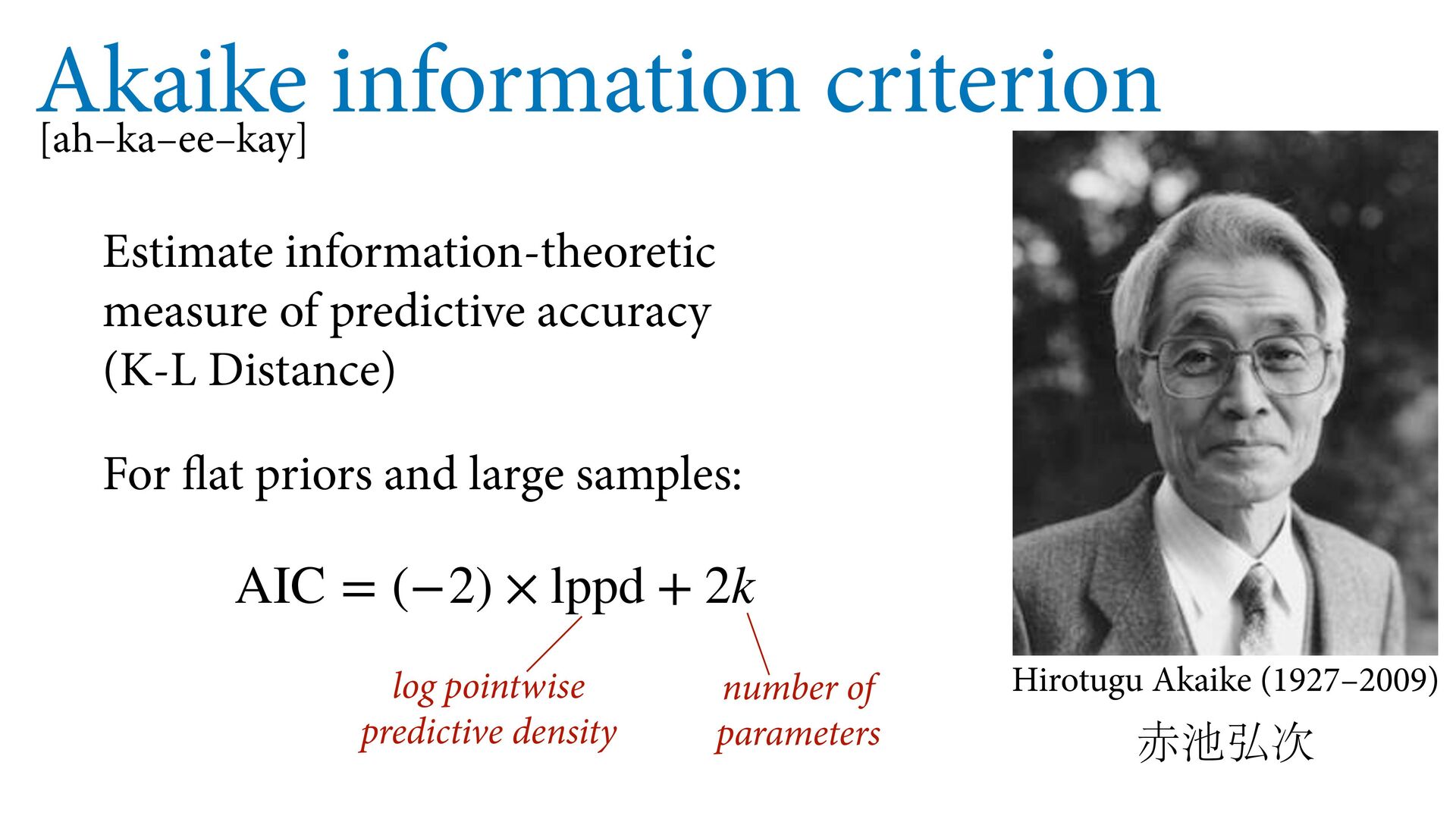
 (K-L Distance) For flat priors and large samples: Hirotugu Akaike (1927–2009)
 [ah–ka–ee–kay] AIC = (−2) × lppd + 2k number of parameters log pointwise predictive density
33. Widely Applicable IC AIC of historical interest now Widely Applicable Information Criterion (WAIC) Sumio Watanabe ( ) 2010 N UIF EBUB HFOFSBUJOH NPEFM .PSF JOUVJUJWFMZ UIF "LBJLF SFTVMU USBEFT PO B TZNNFUSZ TBNQMF BOE PVUPGTBNQMF ćF UXP TBNQMFT BSF FYDIBOHFBCMF ćFZ DPNF GSPN UIF TBNF TTVNQUJPO <OPU ĕOJTIFE  OFFE UP SFMBUF %JO BOE %PVU UP %CBS UP EFMJWFS TPNF JOUVJUJPO IJT KVTU JTOU JOUVJUJWF> P XF DPNQVUF 8"*$ 6OGPSUVOBUFMZ JUT HFOFSBMJUZ DPNFT BU UIF FYQFOTF PG B NPSF E GPSNVMB #VU SFBMMZ JU KVTU IBT UXP QJFDFT BOE ZPV DBO DPNQVUF CPUI EJSFDUMZ MFT GSPN UIF QPTUFSJPS EJTUSJCVUJPO 8"*$ JT KVTU UIF MPHQPTUFSJPSQSFEJDUJWF QE QBHF  UIBU XF DBMDVMBUFE FBSMJFS QMVT B QFOBMUZ QSPQPSUJPOBM UP UIF WBSJBODF FSJPS QSFEJDUJPOT 8"*$(Z, Θ) = − MQQE − J WBS Θ MPH Q(ZJ|Θ) QFOBMUZ UFSN UIF PCTFSWBUJPOT BOE Θ JT UIF QPTUFSJPS EJTUSJCVUJPO ćF QFOBMUZ UFSN NFBOT IF WBSJBODF JO MPHQSPCBCJMJUJFT GPS FBDI PCTFSWBUJPO J BOE UIFO TVN VQ UIFTF P HFU UIF UPUBM QFOBMUZw 4P ZPV DBO UIJOL PG FBDI PCTFSWBUJPO BT IBWJOH JUT PXO Very similar to PSIS score, but no automatic diagnostics
34. 1 2 3 4 5 150 200 250 300 polynomial terms prediction error 1 2 3 4 5 30 35 40 45 50 55 60 polynomial terms log pointwise predictive density WAIC PSIS lppd leave-one-out
 cross-validation
35. Overfit Underfit WAIC,PSIS,CV measure overfitting Regularization manages overfitting None directly address causal inference All important to understanding how statistical inference works
36. Model Mis-selection Do not use predictive criteria (WAIC, PSIS, CV) to choose a causal estimate Predictive criteria actually prefer confounds & colliders Example: Plant growth experiment H0 H1 T F
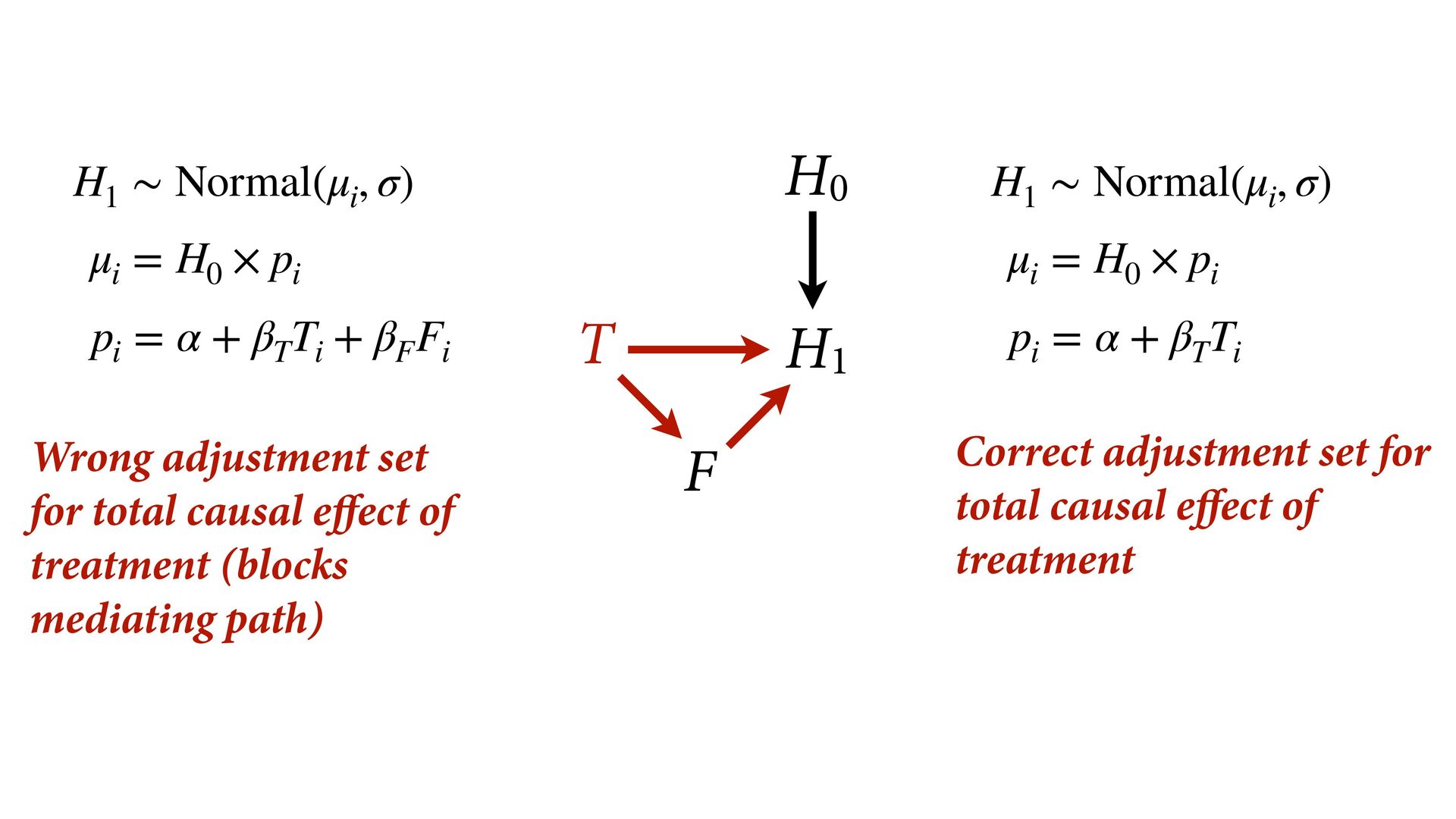
37. H 1 ∼ Normal(μ i , σ) μ i = H 0 × p i p i = α + β T T i + β F F i H 1 ∼ Normal(μ i , σ) μ i = H 0 × p i p i = α + β T T i Wrong adjustment set for total causal effect of treatment (blocks mediating path) Correct adjustment set for total causal effect of treatment H0 H1 T F
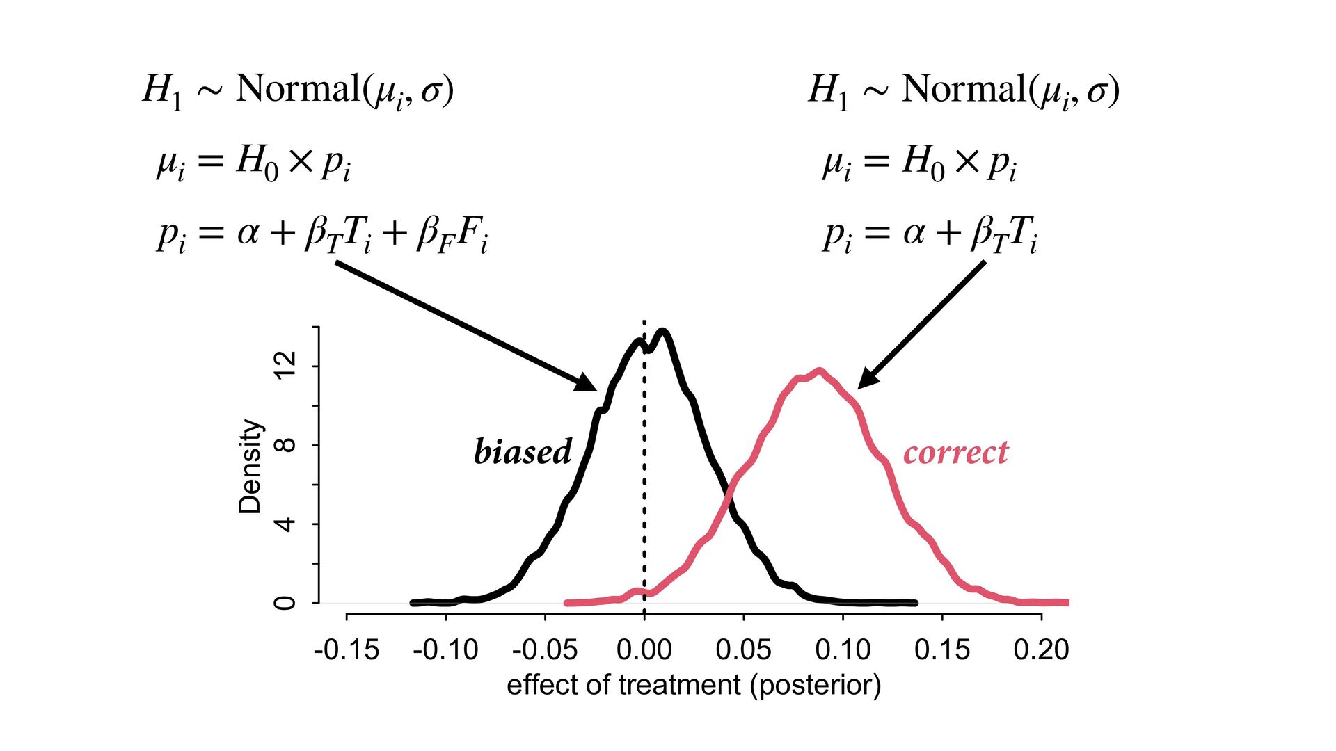
38. H 1 ∼ Normal(μ i , σ) μ i = H 0 × p i p i = α + β T T i + β F F i H 1 ∼ Normal(μ i , σ) μ i = H 0 × p i p i = α + β T T i -0.15 -0.10 -0.05 0.00 0.05 0.10 0.15 0.20 0 4 8 12 effect of treatment (posterior) Density correct biased
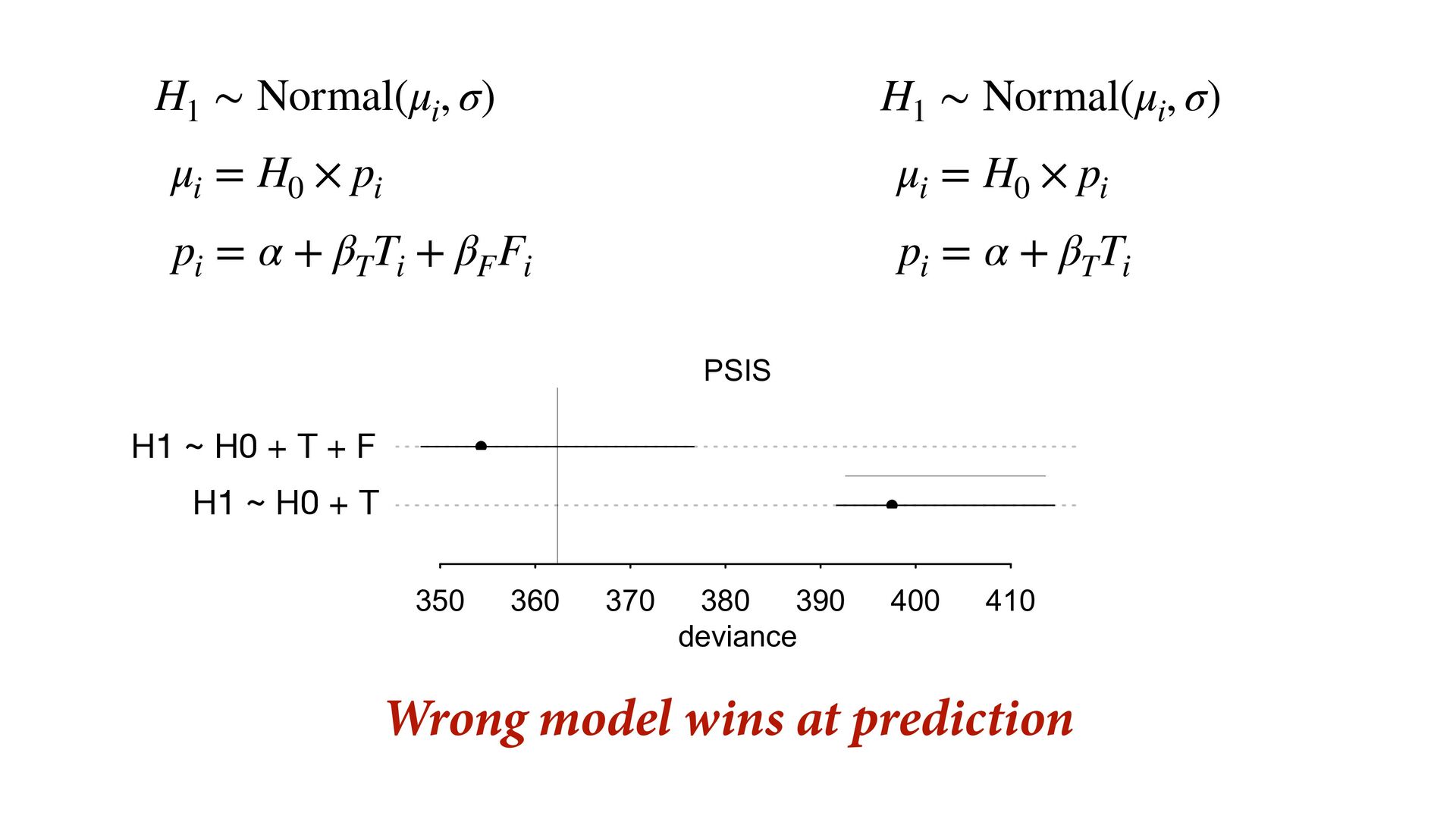
39. H 1 ∼ Normal(μ i , σ) μ i = H 0 × p i p i = α + β T T i + β F F i H 1 ∼ Normal(μ i , σ) μ i = H 0 × p i p i = α + β T T i m6.8 m6.7 350 360 370 380 390 400 410 deviance PSIS H1 ~ H0 + T + F H1 ~ H0 + T Wrong model wins at prediction
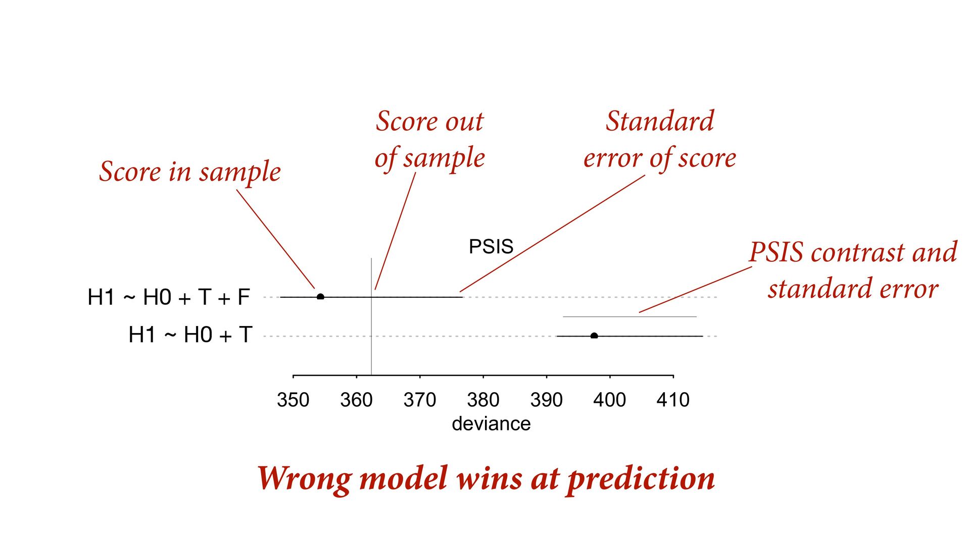
40. m6.8 m6.7 350 360 370 380 390 400 410 deviance PSIS H1 ~ H0 + T + F H1 ~ H0 + T Wrong model wins at prediction Score in sample Score out of sample Standard error of score PSIS contrast and standard error
41. 1.2 1.4 1.6 1.8 2.0 growth no fungus yo fungus treatment control H0 H1 T F Why does the wrong model win at prediction?
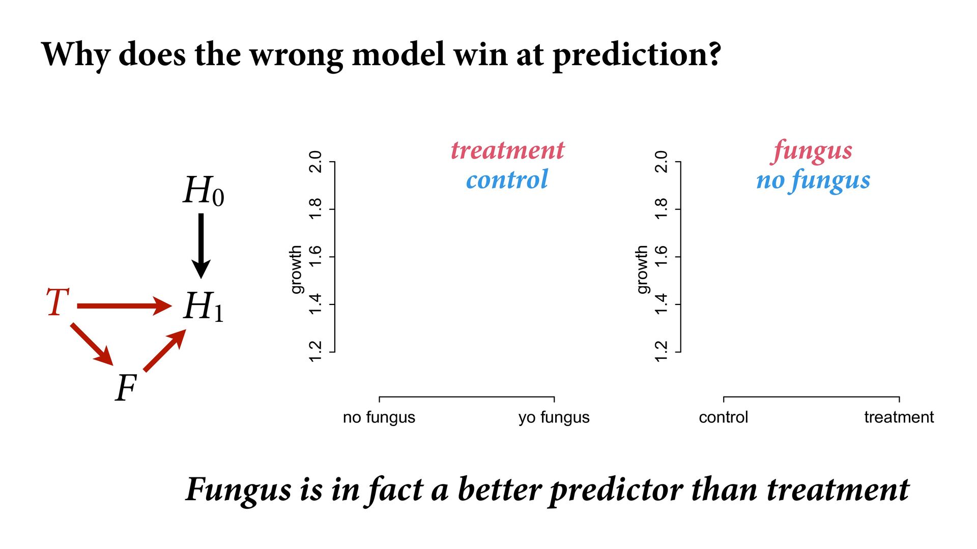
42. 1.2 1.4 1.6 1.8 2.0 growth no fungus yo fungus 1.2 1.4 1.6 1.8 2.0 growth control treatment treatment control fungus no fungus H0 H1 T F Why does the wrong model win at prediction? Fungus is in fact a better predictor than treatment
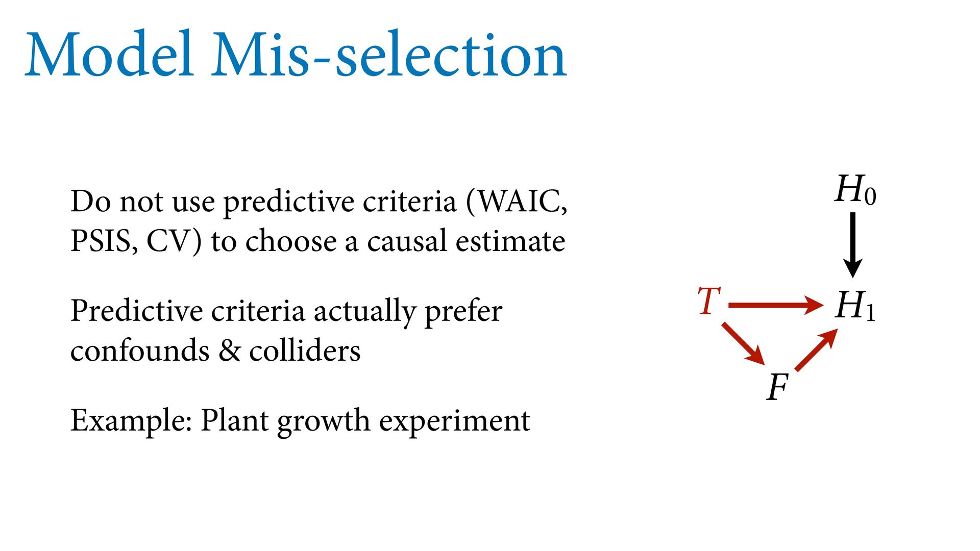
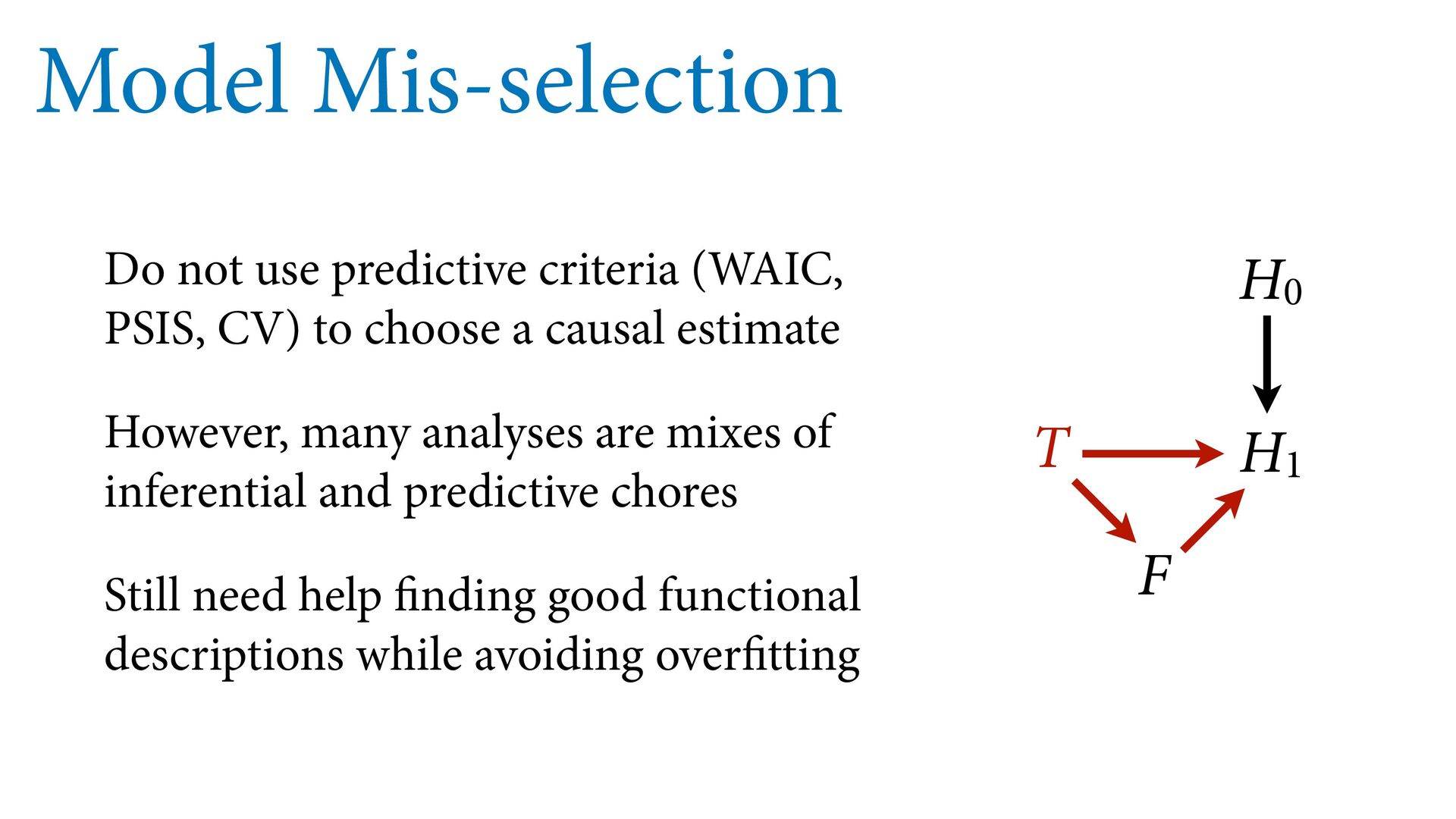
43. Model Mis-selection Do not use predictive criteria (WAIC, PSIS, CV) to choose a causal estimate However, many analyses are mixes of inferential and predictive chores Still need help finding good functional descriptions while avoiding overfitting H0 H1 T F
44. Outliers & Robust Regression Some points are more influential than others “Outliers”: Observations in the tails of predictive distribution Outliers indicate predictions are possibly overconfident, unreliable The model doesn’t expect enough variation -4 -2 0 2 4 -4 -2 0 2 4 -4 -2 0 2 4 -4 -2 0 2 4
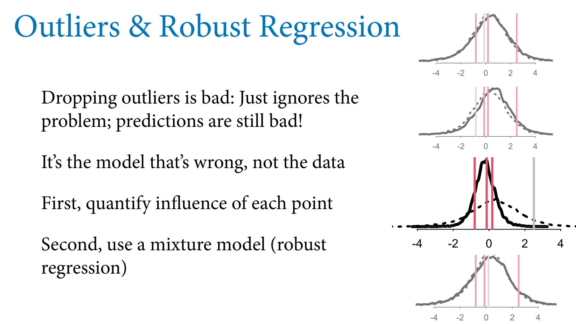
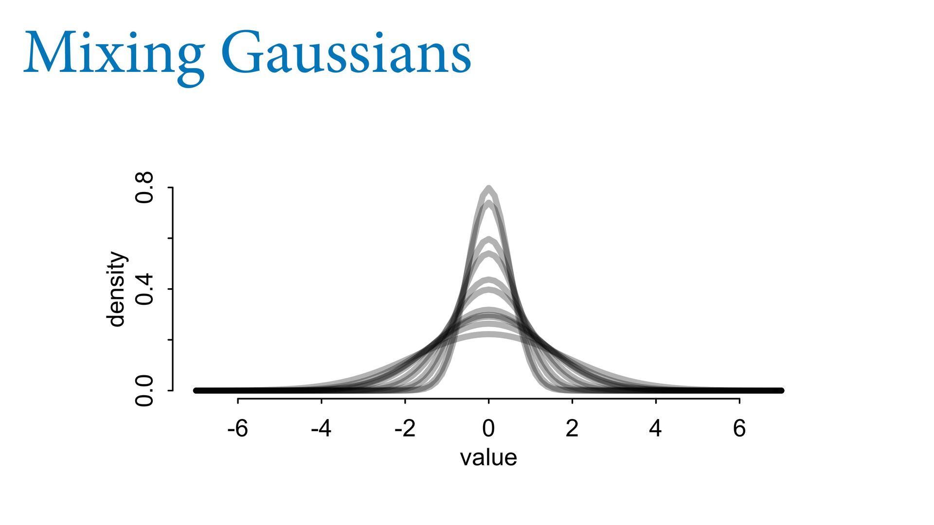
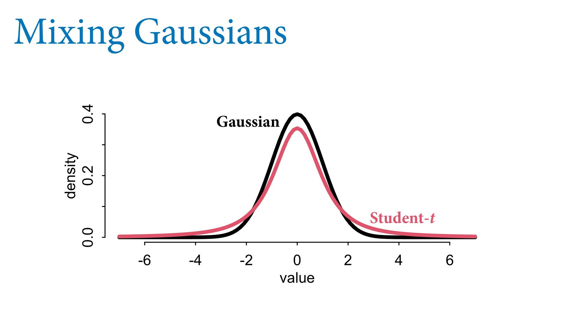
45. Outliers & Robust Regression Dropping outliers is bad: Just ignores the problem; predictions are still bad! It’s the model that’s wrong, not the data First, quantify influence of each point Second, use a mixture model (robust regression) -4 -2 0 2 4 -4 -2 0 2 4 -4 -2 0 2 4 -4 -2 0 2 4
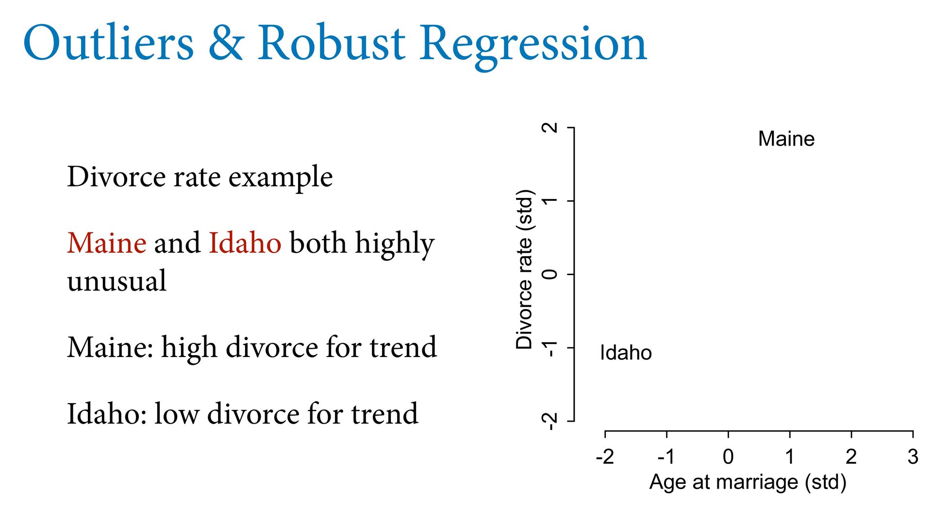
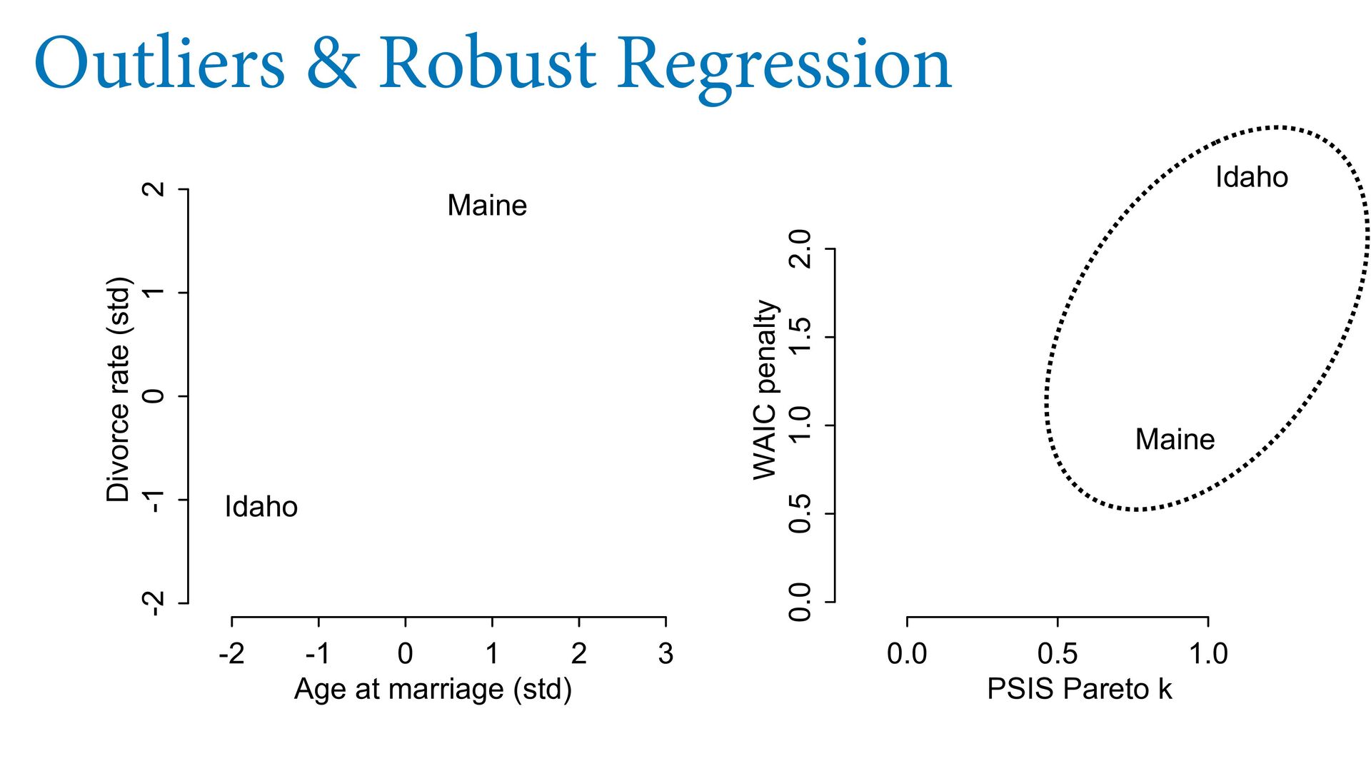
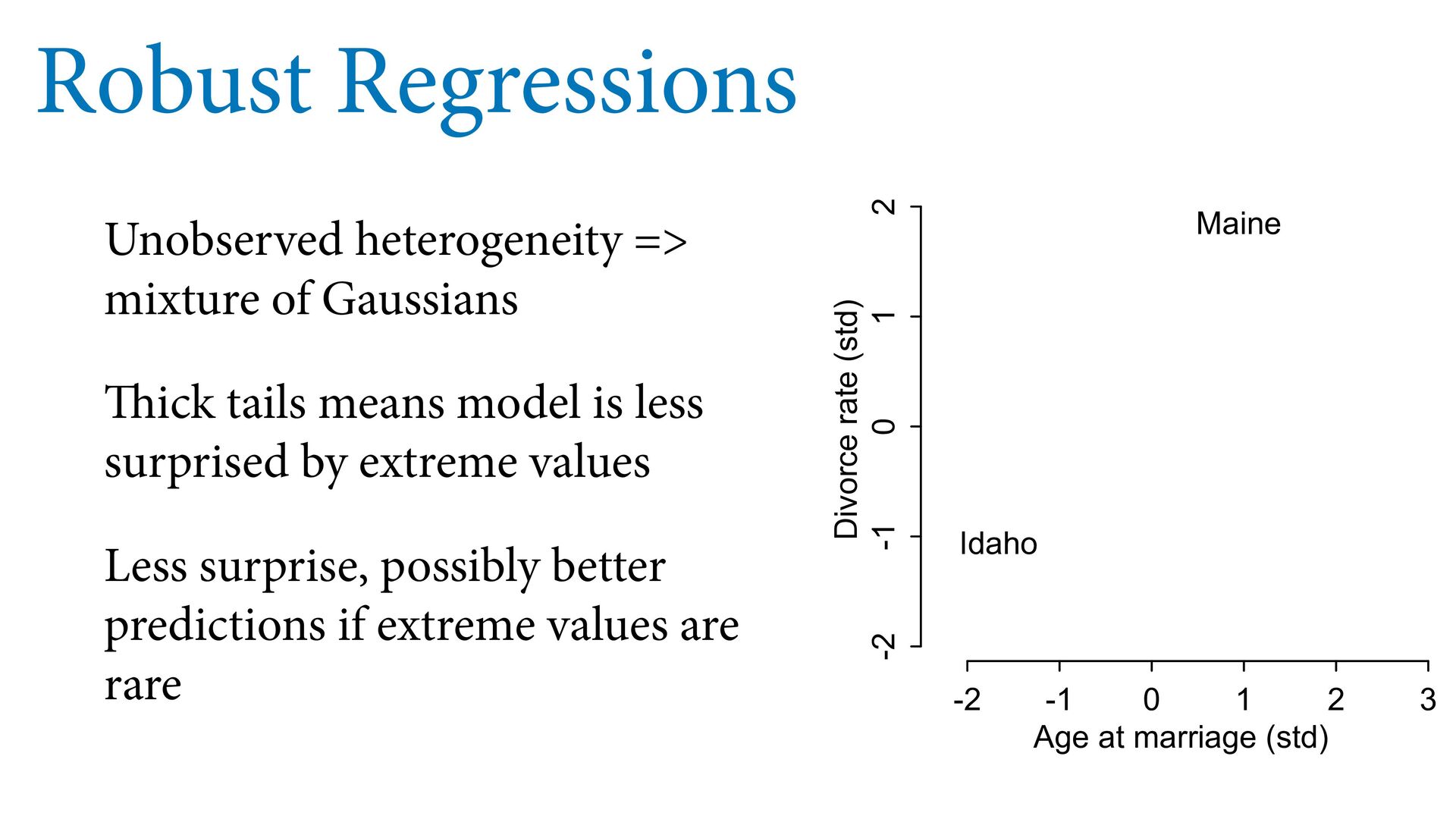
46. Outliers & Robust Regression Divorce rate example Maine and Idaho both highly unusual Maine: high divorce for trend Idaho: low divorce for trend -2 -1 0 1 2 3 -2 -1 0 1 2 Age at marriage (std) Divorce rate (std) Idaho Maine
47. Outliers & Robust Regression Quantify influence: PSIS k statistic WAIC penalty term (“effective number of parameters”) 0.0 0.5 1.0 0.0 0.5 1.0 1.5 2.0 PSIS Pareto k WAIC penalty Idaho Maine
48. Outliers & Robust Regression 0.0 0.5 1.0 0.0 0.5 1.0 1.5 2.0 PSIS Pareto k WAIC penalty Idaho Maine -2 -1 0 1 2 3 -2 -1 0 1 2 Age at marriage (std) Divorce rate (std) Idaho Maine
49. Mixing Gaussians -6 -4 -2 0 2 4 6 0.0 0.4 0.8 value density
50. Mixing Gaussians -6 -4 -2 0 2 4 6 0.0 0.2 0.4 value density Student-t Gaussian
51. m5.3 <- quap( alist( D ~ dnorm( mu , sigma ) , mu <- a + bM*M + bA*A , a ~ dnorm( 0 , 0.2 ) , bM ~ dnorm( 0 , 0.5 ) , bA ~ dnorm( 0 , 0.5 ) , sigma ~ dexp( 1 ) ) , data = dat ) m5.3t <- quap( alist( D ~ dstudent( 2 , mu , sigma ) , mu <- a + bM*M + bA*A , a ~ dnorm( 0 , 0.2 ) , bM ~ dnorm( 0 , 0.5 ) , bA ~ dnorm( 0 , 0.5 ) , sigma ~ dexp( 1 ) ) , data = dat )
52. m5.3 <- quap( alist( D ~ dnorm( mu , sigma ) , mu <- a + bM*M + bA*A , a ~ dnorm( 0 , 0.2 ) , bM ~ dnorm( 0 , 0.5 ) , bA ~ dnorm( 0 , 0.5 ) , sigma ~ dexp( 1 ) ) , data = dat ) m5.3t <- quap( alist( D ~ dstudent( 2 , mu , sigma ) , mu <- a + bM*M + bA*A , a ~ dnorm( 0 , 0.2 ) , bM ~ dnorm( 0 , 0.5 ) , bA ~ dnorm( 0 , 0.5 ) , sigma ~ dexp( 1 ) ) , data = dat ) -1.2 -1.0 -0.8 -0.6 -0.4 -0.2 0.0 0.0 0.5 1.0 1.5 2.0 2.5 3.0 bA (effect of age of marriage) Density Student-t model Gaussian model
53. Robust Regressions Unobserved heterogeneity => mixture of Gaussians Thick tails means model is less surprised by extreme values Less surprise, possibly better predictions if extreme values are rare -2 -1 0 1 2 3 -2 -1 0 1 2 Age at marriage (std) Divorce rate (std) Idaho Maine
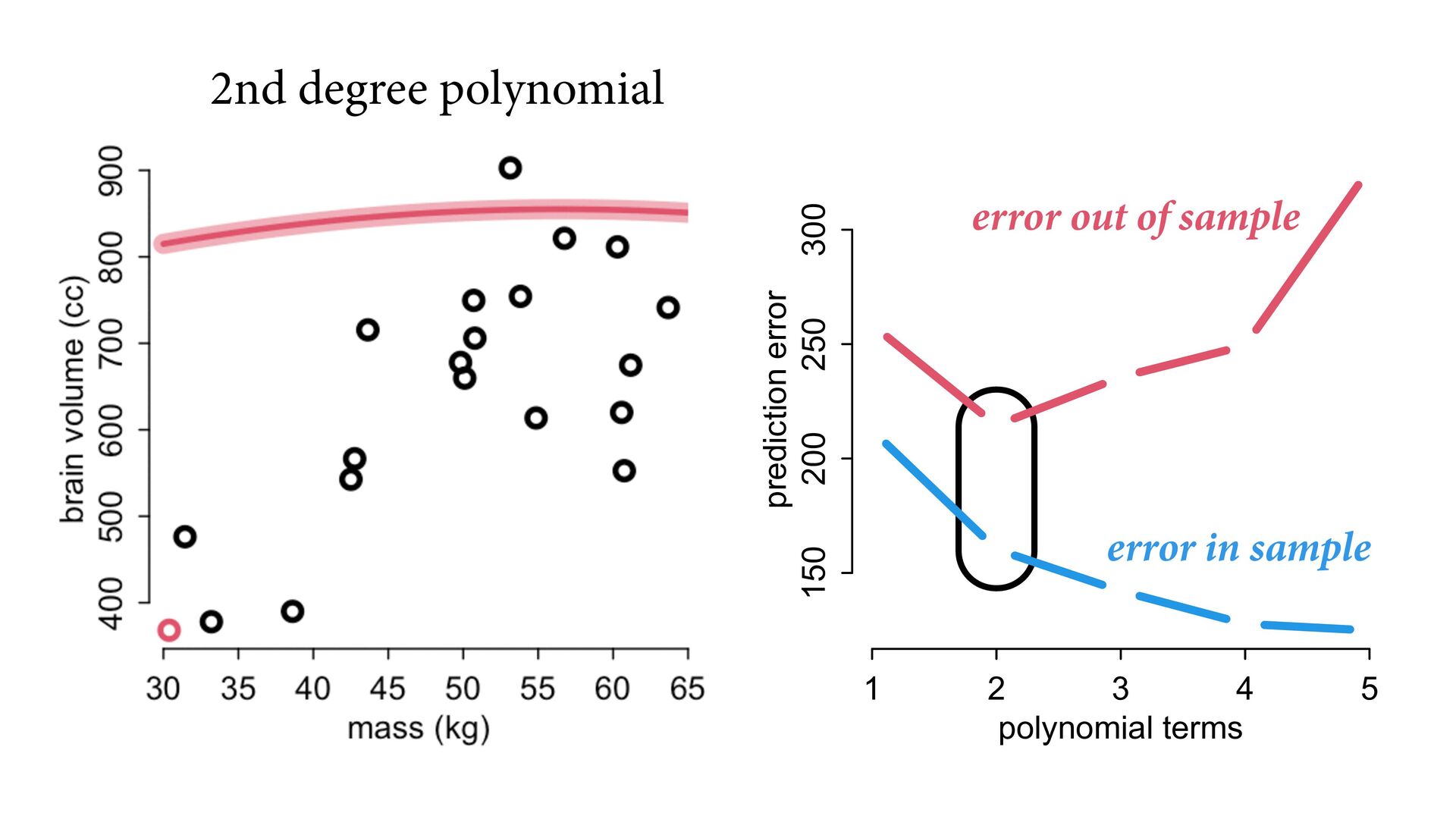
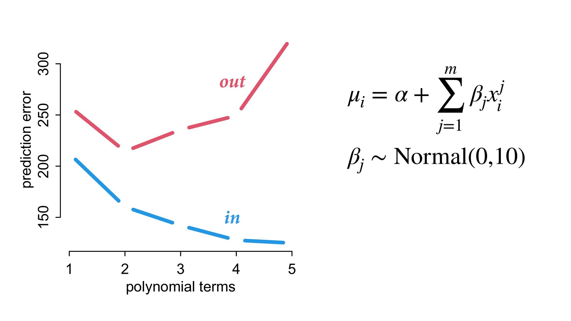
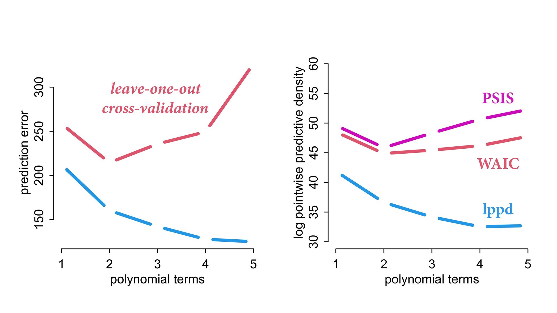
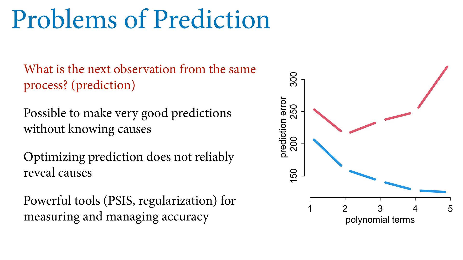
54. Problems of Prediction What is the next observation from the same process? (prediction) Possible to make very good predictions without knowing causes Optimizing prediction does not reliably reveal causes Powerful tools (PSIS, regularization) for measuring and managing accuracy 1 2 3 4 5 150 200 250 300 polynomial terms prediction error
55. Course Schedule Week 1 Bayesian inference Chapters 1, 2, 3 Week 2 Linear models & Causal Inference Chapter 4 Week 3 Causes, Confounds & Colliders Chapters 5 & 6 Week 4 Overfitting / MCMC Chapters 7, 8, 9 Week 5 Generalized Linear Models Chapters 10, 11 Week 6 Integers & Other Monsters Chapters 11 & 12 Week 7 Multilevel models I Chapter 13 Week 8 Multilevel models II Chapter 14 Week 9 Measurement & Missingness Chapter 15 Week 10 Generalized Linear Madness Chapter 16 https://github.com/rmcelreath/stat_rethinking_2022