Statistical Rethinking 2022 Lecture 20

Course materials: https://github.com/rmcelreath/stat_rethinking_2022

Transcript

1. Statistical Rethinking 20: Horoscopes 2022
3. Horoscope of Prince Iskandar, grandson of Tamerlane
10. * *** **
11. Stargazing Fortune telling frameworks: (1) From vague facts, vague advice (2) Exaggerated importance Applies to astrologers and statisticians Valid vague advice exists, not sufficient *** ** * * p < 0.05 p < 0.001 p < 0.01
12. Stargazing Statistical procedures acquire meaning from scientific models Cannot offload subjective responsibility to an objective procedure Many subjective responsibilities
13. A Typical Scientific Laboratory
14. A Typical Scientific Laboratory Quality of theory Reliable Procedures/Code Quality of data analysis Documentation Reporting Quality of Data
15. @StuartJRitchie Planning
16. @StuartJRitchie Planning Working DATA ANALYSIS IN REALITY DATA ANALYSIS
 IN THE MOVIES
17. @StuartJRitchie DATA ANALYSIS IN REALITY DATA ANALYSIS
 IN THE MOVIES Planning Working Reporting
18. Planning Goal setting Theory building Justified sampling plan Justified analysis plan Documentation Open software & data formats @StuartJRitchie
19. Planning Goal setting – What for? Estimands Theory building Justified sampling plan Justified analysis plan Documentation Open software & data formats ESTIMAND Ingredients 150g unsalted butter 150g chocolate pieces 150g all-purpose flour 1/2 tsp baking powder 1/2 tsp baking soda 200g brown sugar 2 large eggs Directions 1. Heat oven to 160C. Grease 1 liter glass baking pan. Line a 450g loaf tin with baking paper. 2. Melt butter and chocolate in a saucepan over low heat. ESTIMATOR ESTIMATE
20. Planning Goal setting – What for? Estimands Theory building – Which assumptions? Justified sampling plan Justified analysis plan Documentation Open software & data formats ESTIMAND Ingredients 150g unsalted butter 150g chocolate pieces 150g all-purpose flour 1/2 tsp baking powder 1/2 tsp baking soda 200g brown sugar 2 large eggs Directions 1. Heat oven to 160C. Grease 1 liter glass baking pan. Line a 450g loaf tin with baking paper. 2. Melt butter and chocolate in a saucepan over low heat. ESTIMATOR ESTIMATE
21. Theory Building Levels of theory building (1) Heuristic causal models (DAGs) (2) Structural causal models (3) Dynamic models (4) Agent-based models G D A u dH dt = H t b H − H t (L t m H ) dL dt = L t (H t b L ) − L t m L
22. Theory Building Heuristic causal models (DAGs) (1) Treatment and outcome (2) Other causes (3) Other effects (4) Unobserved causes G D A u
23. Theory Building Heuristic causal models (DAGs) (1) Treatment and outcome (2) Other causes (3) Other effects (4) Unobserved causes G A
24. Theory Building Heuristic causal models (DAGs) (1) Treatment and outcome (2) Other causes (3) Other effects (4) Unobserved causes G D A
25. Theory Building Heuristic causal models (DAGs) (1) Treatment and outcome (2) Other causes (3) Other effects (4) Unobserved causes G D A
26. Theory Building Heuristic causal models (DAGs) (1) Treatment and outcome (2) Other causes (3) Other effects (4) Unobserved causes G D A u
27. Planning Goal setting – What for? Estimands Theory building – Which assumptions? Justified sampling plan – Which data? Justified analysis plan Documentation Open software & data formats ESTIMAND Ingredients 150g unsalted butter 150g chocolate pieces 150g all-purpose flour 1/2 tsp baking powder 1/2 tsp baking soda 200g brown sugar 2 large eggs Directions 1. Heat oven to 160C. Grease 1 liter glass baking pan. Line a 450g loaf tin with baking paper. 2. Melt butter and chocolate in a saucepan over low heat. ESTIMATOR ESTIMATE
28. Planning Goal setting – What for? Estimands Theory building – Which assumptions? Justified sampling plan – Which data? Justified analysis plan – Which golems? Documentation Open software & data formats ESTIMAND Ingredients 150g unsalted butter 150g chocolate pieces 150g all-purpose flour 1/2 tsp baking powder 1/2 tsp baking soda 200g brown sugar 2 large eggs Directions 1. Heat oven to 160C. Grease 1 liter glass baking pan. Line a 450g loaf tin with baking paper. 2. Melt butter and chocolate in a saucepan over low heat. ESTIMATOR ESTIMATE
29. Planning Goal setting – What for? Estimands Theory building – Which assumptions? Justified sampling plan – Which data? Justified analysis plan – Which golems? Documentation – How did it happen? Open software & data formats ESTIMAND Ingredients 150g unsalted butter 150g chocolate pieces 150g all-purpose flour 1/2 tsp baking powder 1/2 tsp baking soda 200g brown sugar 2 large eggs Directions 1. Heat oven to 160C. Grease 1 liter glass baking pan. Line a 450g loaf tin with baking paper. 2. Melt butter and chocolate in a saucepan over low heat. ESTIMATOR ESTIMATE
30. Planning Goal setting – What for? Estimands Theory building – Which assumptions? Justified sampling plan – Which data? Justified analysis plan – Which golems? Documentation – How did it happen? Open software & data formats
31. Pre-Registration Pre-registration: Prior public documentation of research design and analysis plan Goal: Make transparent which decisions are sample-dependent Does little to improve data analysis Lots of pre-registered causal salad @StuartJRitchie
33. Working Control Incremental testing Documentation Review DATA ANALYSIS IN REALITY DATA ANALYSIS
 IN THE MOVIES
34. Express theory as probabilistic program Prove planned analysis could work (conditionally) Test pipeline on synthetic data Run pipeline on empirical data 1 2 3 4 entire history open
35. Professional Norms Dangerous lack of professional norms in scientific computing Often impossible to figure out what was done Often impossible to know if code works as intended Like pipetting by mouth
36. Research Engineering Control: Versioning, back-up, accountability Incremental testing: Piece by piece Documentation: Comment everything Review: 4 eyes on code and materials
37. Research Engineering Control: Versioning, back-up, accountability Incremental testing: Piece by piece Documentation: Comment everything Review: 4 eyes on code and materials
38. Versioning and Testing Version control: Database of changes to project files, managed history Testing: Incremental milestones, test each before moving to next
41. Versioning and Testing Most researchers don’t need all git’s features But do: Commit changes after each milestone
 Maintain test code in project Do not: Replace raw data with processed data
42. More on Testing Complex analyses must be built in steps Test each step Social networks lecture (#15) as example Milestones:
 (1) Synthetic data simulation
 (2) Dyadic reciprocity model
 (3) Add generalized giving/receiving
 (4) Add wealth, association index
43. https://github.com/stan-dev/math 5.1 MB of library code 8.2 MB of test code
45. Documentation & reports Simulation code Validation code Analysis code Sharable data Template data Stan model, full Stan model, milestone 1
47. https://datacarpentry.org/
50. https://www.theverge.com/2020/8/6/21355674
51. https://www.theverge.com/2020/8/6/21355674 Careful primary data entry, okay with rules, tests Never process data in Excel; use code
52. PAUSE
53. Reporting Sharing materials Describing methods Describing data Describing results Making decisions
54. Sharing Materials The paper is an advertisement; the data and its analysis are the product Make code and data available through a link, not “by request” Some data not shareable; code always shareable Archived code & data will be required Culina et al 2020 Low availability of code in ecology: A call for urgent action
55. Describing Methods Minimal information: (1) Math-stats notation of stat model (2) Explanation of how (1) provides estimand (3) Algorithm used to produce estimate (4) Diagnostics, code tests (5) Cite software packages log(λ AB ) = α + T AB + G A + R B G AB ∼ Poisson(λ AB ) G BA ∼ Poisson(λ BA ) log(λ BA ) = α + T BA + G B + R A ( T AB T BA ) ∼ MVNormal [ 0 0] , [ σ2 ρσ2 ρσ2 σ2 ] ρ ∼ LKJCorr(2) σ ∼ Exponential(1) α ∼ Normal(0,1) ( G A R A ) ∼ MVNormal ([ 0 0] , R GR , S GR ) R GR ∼ LKJCorr(2) S GR ∼ Exponential(1)
56. To estimate the reciprocity within dyads, we model the correlation within dyads in giving, using a multilevel mixed-membership model (textbook citation). To control for confounding from generalized giving and receiving, as indicated by the DAG in the previous section, we stratify giving and receiving by household. The full model with priors is presented at right. We estimated the posterior distribution using Hamiltonian Monte Carlo as implemented in Stan version 2.29. We validated the model on simulated data and assessed convergence by inspection of trace plots, R-hat values, and effective sample sizes. Diagnostics are reported in Appendix B and all results can be replicated using the code available at LINK. log(λ AB ) = α + T AB + G A + R B G AB ∼ Poisson(λ AB ) G BA ∼ Poisson(λ BA ) log(λ BA ) = α + T BA + G B + R A ( T AB T BA ) ∼ MVNormal [ 0 0] , [ σ2 ρσ2 ρσ2 σ2 ] ρ ∼ LKJCorr(2) σ ∼ Exponential(1) α ∼ Normal(0,1) ( G A R A ) ∼ MVNormal ([ 0 0] , R GR , S GR ) R GR ∼ LKJCorr(2) S GR ∼ Exponential(1)
57. To estimate the reciprocity within dyads, we model the correlation within dyads in giving, using a multilevel mixed-membership model (textbook citation). To control for confounding from generalized giving and receiving, as indicated by the DAG in the previous section, we stratify giving and receiving by household. The full model with priors is presented at right. We estimated the posterior distribution using Hamiltonian Monte Carlo as implemented in Stan version 2.29. We validated the model on simulated data and assessed convergence by inspection of trace plots, R-hat values, and effective sample sizes. Diagnostics are reported in Appendix B and all results can be replicated using the code available at LINK. log(λ AB ) = α + T AB + G A + R B G AB ∼ Poisson(λ AB ) G BA ∼ Poisson(λ BA ) log(λ BA ) = α + T BA + G B + R A ( T AB T BA ) ∼ MVNormal [ 0 0] , [ σ2 ρσ2 ρσ2 σ2 ] ρ ∼ LKJCorr(2) σ ∼ Exponential(1) α ∼ Normal(0,1) ( G A R A ) ∼ MVNormal ([ 0 0] , R GR , S GR ) R GR ∼ LKJCorr(2) S GR ∼ Exponential(1)
58. To estimate the reciprocity within dyads, we model the correlation within dyads in giving, using a multilevel mixed-membership model (textbook citation). To control for confounding from generalized giving and receiving, as indicated by the DAG in the previous section, we stratify giving and receiving by household. The full model with priors is presented at right. We estimated the posterior distribution using Hamiltonian Monte Carlo as implemented in Stan version 2.29. We validated the model on simulated data and assessed convergence by inspection of trace plots, R-hat values, and effective sample sizes. Diagnostics are reported in Appendix B and all results can be replicated using the code available at LINK. log(λ AB ) = α + T AB + G A + R B G AB ∼ Poisson(λ AB ) G BA ∼ Poisson(λ BA ) log(λ BA ) = α + T BA + G B + R A ( T AB T BA ) ∼ MVNormal [ 0 0] , [ σ2 ρσ2 ρσ2 σ2 ] ρ ∼ LKJCorr(2) σ ∼ Exponential(1) α ∼ Normal(0,1) ( G A R A ) ∼ MVNormal ([ 0 0] , R GR , S GR ) R GR ∼ LKJCorr(2) S GR ∼ Exponential(1)
59. To estimate the reciprocity within dyads, we model the correlation within dyads in giving, using a multilevel mixed-membership model (textbook citation). To control for confounding from generalized giving and receiving, as indicated by the DAG in the previous section, we stratify giving and receiving by household. The full model with priors is presented at right. We estimated the posterior distribution using Hamiltonian Monte Carlo as implemented in Stan version 2.29. We validated the model on simulated data and assessed convergence by inspection of trace plots, R-hat values, and effective sample sizes. Diagnostics are reported in Appendix B and all results can be replicated using the code available at LINK. log(λ AB ) = α + T AB + G A + R B G AB ∼ Poisson(λ AB ) G BA ∼ Poisson(λ BA ) log(λ BA ) = α + T BA + G B + R A ( T AB T BA ) ∼ MVNormal [ 0 0] , [ σ2 ρσ2 ρσ2 σ2 ] ρ ∼ LKJCorr(2) σ ∼ Exponential(1) α ∼ Normal(0,1) ( G A R A ) ∼ MVNormal ([ 0 0] , R GR , S GR ) R GR ∼ LKJCorr(2) S GR ∼ Exponential(1)
60. Justify Priors “Priors were chosen through prior predictive simulation so that pre- data predictions span the range of scientifically plausible outcomes. In the results, we explicitly compare the posterior distribution to the prior, so that the impact of the sample is obvious.” 0.0 0.2 0.4 0.6 0.8 1.0 0.0 0.5 1.0 1.5 phylogenetic distance covariance prior posterior B posterior BMG
61. Justifying Methods Naive reviewers: “Good science doesn’t need complex stats” Causal model often requires complexity Big data => unit heterogeneity Ethical responsibility to do our best Change discussion from statistics to causal models “Pooh?” said Piglet. “Yes, Piglet?” said Pooh. “27417 parameters,” said Piglet. “Oh, bother,” said Pooh.
62. Justifying Methods Write for the editor, not the reviewer Find other papers in discipline/journal that have used Bayesian methods or similar models (Bayesian or not) Explain results in Bayesian terms, show densities, cite disciplinary guides Bayes is ancient, normative, often the only practical way to estimate complex models “Pooh?” said Piglet. “Yes, Piglet?” said Pooh. “27417 parameters,” said Piglet. “Oh, bother,” said Pooh.
63. Describing Data 1k observations of 1 person
 -vs-
 1 observation of each of 1k people “Effective” sample size function of estimand and hierarchical structure Variables measured at which levels? Missing values!
64. Describing Results Estimands, marginal causal effects Warn against causal interpretation of control variables (Table 2 fallacy) Densities better than intervals; Sample realizations often better than densities Figures assist comparisons reciprocity give-receive -1.0 -0.5 0.0 0.5 1.0 0 5 10 15 correlation within dyads Density -1.0 -0.5 0.0 0.5 1.0 0.0 0.5 1.0 1.5 2.0 correlation giving-receiving Density receiving giving -0.4 -0.2 0.0 0.2 0.4 0.6 0.8 0 1 2 3 4 5 effect of wealth Density
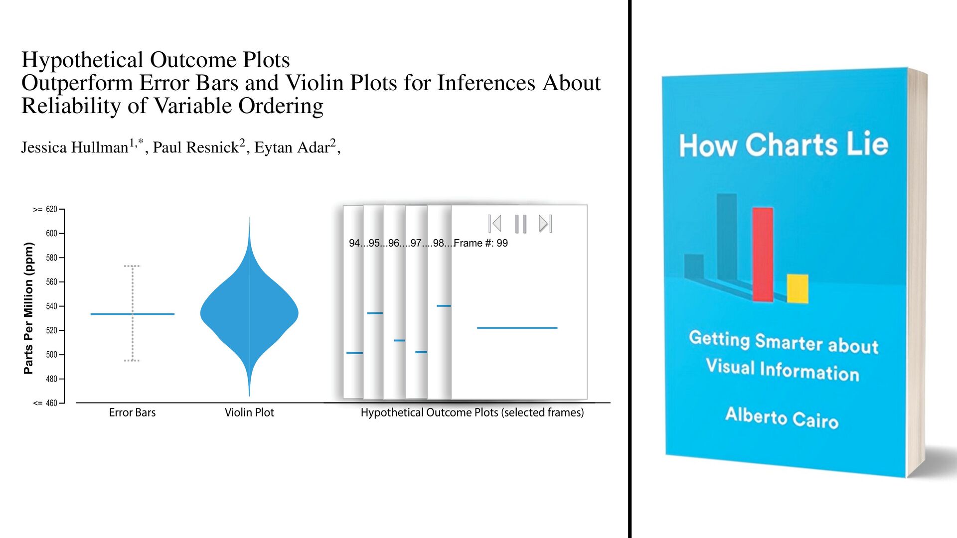
65. Hypothetical Outcome Plots Outperform Error Bars and Violin Plots for Inferences About Reliability of Variable Ordering Jessica Hullman1,*, Paul Resnick2, Eytan Adar2, 1 Information School, University of Washington, Seattle, WA, USA 2 School of Information, University of Michigan, Ann Arbor, MI, USA * jhullman@uw.edu Abstract Many visual depictions of probability distributions, such as error bars, are difficult for users to accurately interpret. We present and study an alternative representation, Hypothetical Outcome Plots (HOPs), that animates a finite set of individual draws. In contrast to the statistical background required to interpret many static representations of distributions, HOPs require relatively little background knowledge to interpret. Instead, HOPs enables viewers to infer properties of the distribution using mental processes like counting and integration. We conducted an experiment comparing HOPs to error bars and violin plots. With HOPs, people made much more accurate judgments about plots of two and three quantities. Accuracy was similar with all three representations for most questions about distributions of a single quantity. 460 480 500 520 540 560 580 600 620 Parts Per Million (ppm) <= >= Error Bars Violin Plot Hypothetical Outcome Plots (selected frames) rames) lected fram s (selec Outcome Plots (s cted f selec Outcome Plots (s Outcome Plo 94...95...96....97....98....Frame #: 99 udy conditions. Error bars convey the mean of a ong with a vertical “error bar” capturing a 95% dea by showing the distribution in a mirrored OPs) present the same distribution as animated
66. Making Decisions Academic research: Communicate uncertainty, conditional on sample & models Industry research: What should we do, given the uncertainty, conditional on sample & models? Also: “Does my boss have any idea what ‘uncertainty’ means, or does he think that’s the refuge of cowards?” POSTERIOR DOGE DECISION DOGE
67. Making Decisions Bayesian decision theory: (1) State costs & benefits of outcomes
 (2) Compute posterior benefits of hypothetical policy choices Simple example in Chapter 3 Can be integrated with dynamic optimization POSTERIOR DOGE DECISION DOGE
68. ME DISCUSSING SCIENCE REFORM SCIENCE
69. 1. Hypothesis Selection! Novel hypotheses! Tested hypotheses! A previously tested hypothesis is selected for replication with probability r, otherwise a novel (untested) hypothesis is selected. Novel hypotheses are true with probability b. ! 1 – r! r! 2. Investigation! T! Real truth of hypothesis! Probability of result! 1 – β α β 1 – α + – 3. Communication! Experimental results are communicated to the scientific community with a probability that depends upon both the experimental result (+, –) and whether the hypothesis was novel (N) or a replication (R). Communicated results join the set of tested hypotheses. Uncommunicated replications revert to their prior status.! 1 – C N– C N– positive results! negative results! 1 – C R+ C R+ New result communicated! New result not communicated! 1 – C R– C R– File drawer! novel! replic.! novel! replic.! True (T)! False (T)! KEY! Interior = true epistemic state ! Exterior = experimental evidence! Unknown! Positive (+)! Negative (–)! General case! General case (+ or –)! F! McElreath & Smaldino. 2015. Replication, communication, and the population dynamics of scientific discovery.
70. 1. Hypothesis Selection! Novel hypotheses! Tested hypotheses! A previously tested hypothesis is selected for replication with probability r, otherwise a novel (untested) hypothesis is selected. Novel hypotheses are true with probability b. ! 1 – r! r! 2. Investigation! T! Real truth of hypothesis! Probability of result! 1 – β α β 1 – α + – 3. Communication! Experimental results are communicated to the scientific community with a probability that depends upon both the experimental result (+, –) and whether the hypothesis was novel (N) or a replication (R). Communicated results join the set of tested hypotheses. Uncommunicated replications revert to their prior status.! 1 – C N– C N– positive results! negative results! 1 – C R+ C R+ New result communicated! New result not communicated! 1 – C R– C R– File drawer! novel! replic.! novel! replic.! True (T)! False (T)! KEY! Interior = true epistemic state ! Exterior = experimental evidence! Unknown! Positive (+)! Negative (–)! General case! General case (+ or –)! F! McElreath & Smaldino. 2015. Replication, communication, and the population dynamics of scientific discovery.
71. 1. Hypothesis Selection! Novel hypotheses! Tested hypotheses! A previously tested hypothesis is selected for replication with probability r, otherwise a novel (untested) hypothesis is selected. Novel hypotheses are true with probability b. ! 1 – r! r! 2. Investigation! T! Real truth of hypothesis! Probability of result! 1 – β α β 1 – α + – 3. Communication! Experimental results are communicated to the scientific community with a probability that depends upon both the experimental result (+, –) and whether the hypothesis was novel (N) or a replication (R). Communicated results join the set of tested hypotheses. Uncommunicated replications revert to their prior status.! 1 – C N– C N– positive results! negative results! 1 – C R+ C R+ New result communicated! New result not communicated! 1 – C R– C R– File drawer! novel! replic.! novel! replic.! True (T)! False (T)! KEY! Interior = true epistemic state ! Exterior = experimental evidence! Unknown! Positive (+)! Negative (–)! General case! General case (+ or –)! F! McElreath & Smaldino. 2015. Replication, communication, and the population dynamics of scientific discovery.
72. 1. Hypothesis Selection! Novel hypotheses! Tested hypotheses! A previously tested hypothesis is selected for replication with probability r, otherwise a novel (untested) hypothesis is selected. Novel hypotheses are true with probability b. ! 1 – r! r! 2. Investigation! T! Real truth of hypothesis! Probability of result! 1 – β α β 1 – α + – 3. Communication! Experimental results are communicated to the scientific community with a probability that depends upon both the experimental result (+, –) and whether the hypothesis was novel (N) or a replication (R). Communicated results join the set of tested hypotheses. Uncommunicated replications revert to their prior status.! 1 – C N– C N– positive results! negative results! 1 – C R+ C R+ New result communicated! New result not communicated! 1 – C R– C R– File drawer! novel! replic.! novel! replic.! True (T)! False (T)! KEY! Interior = true epistemic state ! Exterior = experimental evidence! Unknown! Positive (+)! Negative (–)! General case! General case (+ or –)! F! McElreath & Smaldino. 2015. Replication, communication, and the population dynamics of scientific discovery.
73. 1. Hypothesis Selection! Novel hypotheses! Tested hypotheses! A previously tested hypothesis is selected for replication with probability r, otherwise a novel (untested) hypothesis is selected. Novel hypotheses are true with probability b. ! 1 – r! r! 2. Investigation! T! Real truth of hypothesis! Probability of result! 1 – β α β 1 – α + – 3. Communication! Experimental results are communicated to the scientific community with a probability that depends upon both the experimental result (+, –) and whether the hypothesis was novel (N) or a replication (R). Communicated results join the set of tested hypotheses. Uncommunicated replications revert to their prior status.! 1 – C N– C N– positive results! negative results! 1 – C R+ C R+ New result communicated! New result not communicated! 1 – C R– C R– File drawer! novel! replic.! novel! replic.! True (T)! False (T)! KEY! Interior = true epistemic state ! Exterior = experimental evidence! Unknown! Positive (+)! Negative (–)! General case! General case (+ or –)! F! McElreath & Smaldino. 2015. Replication, communication, and the population dynamics of scientific discovery.
74. Serra-Garcia & Gneezy 2021 Nonreplicable publications are cited more than replicable ones Replicated Not
 Replicated Replicated Replicated Not
 Replicated Not
 Replicated
75. Page 162 -2 -1 0 1 2 3 -3 -2 -1 0 1 2 3 newsworthiness trustworthiness 200 papers/proposals No correlation
76. -2 -1 0 1 2 3 -3 -2 -1 0 1 2 3 newsworthiness trustworthiness Select top 10% Page 162
77. -2 -1 0 1 2 3 -3 -2 -1 0 1 2 3 newsworthiness trustworthiness Correlation = –0.77 Page 162
78. -2 -1 0 1 2 3 -3 -2 -1 0 1 2 3 newsworthiness trustworthiness Page 162 N P T published newsworthy trustworthy
79. Horoscopes for Research No one knows how research works But many easy fixes at hand (1) No stats without associated causal model
 (2) Prove that your code works (in principle)
 (3) Share as much as possible
 (4) Beware proxies of research quality Many things you dislike about academia were once well-intentioned reforms Replicated Not
 Replicated
80. END