Spatial Sound Synthesis with Loudspeakers

Talk I gave at the EAA Winter School 2013 in Meran, Italy on the theoretical basis of Sound Field Synthesis techniques like higher-order Ambisonics (HOA) and Wave Field Synthesis (WFS).

Transcript

1. Spatial Sound Synthesis with Loudspeakers Sascha Spors 1 and Franz Zotter 2 1Universität Rostock, Institute of Communications Engineering 2University of Music and Performing Arts Graz, Institute of Electronic Music and Acoustics
2. Problem Statement Perfect synthesis of the virtual source s(x, t) within the listening area V by loudspeakers (secondary sources) placed on the border ∂V s(x, t) ∂V V virtual source • assumed to result in authentic reproduction of original scene • frequency dependent weighting of secondary sources ⇒ driving signal Spors, Zotter | Sound Field Synthesis | Overview 1
3. Overview [from W. Snow, Basic Principles of Stereophonic Sound, 1955] • thorough review of the underlying physical problem • Higher-Order Ambisonics and Wave Field Synthesis Spors, Zotter | Sound Field Synthesis | Overview 2
4. Conventions Fourier-Transformation with respect to time t S(ω, x) = ∞ −∞ s(t, x)e−iωt dt Fourier-Transformation with respect to position vector x = [x y z]T ˜ S(ω, k) = ∞ −∞ S(ω, x)e+i k,x dxdydz Example: 3D free-field Green’s function (acoustic point source) g0,3D (x|x0 , t) = 1 4π δ(t − x−x0 c ) x − x0 G0,3D (x|x0 , ω) = 1 4π e−i ω c x−x0 x − x0 ˜ G0,3D (k|x0 , ω) = 1 k 2 − (ω c )2 ei k,x0 Caution: Different definitions of the spatio-temporal Fourier-Transformation in the literature Spors, Zotter | Sound Field Synthesis | Overview 3
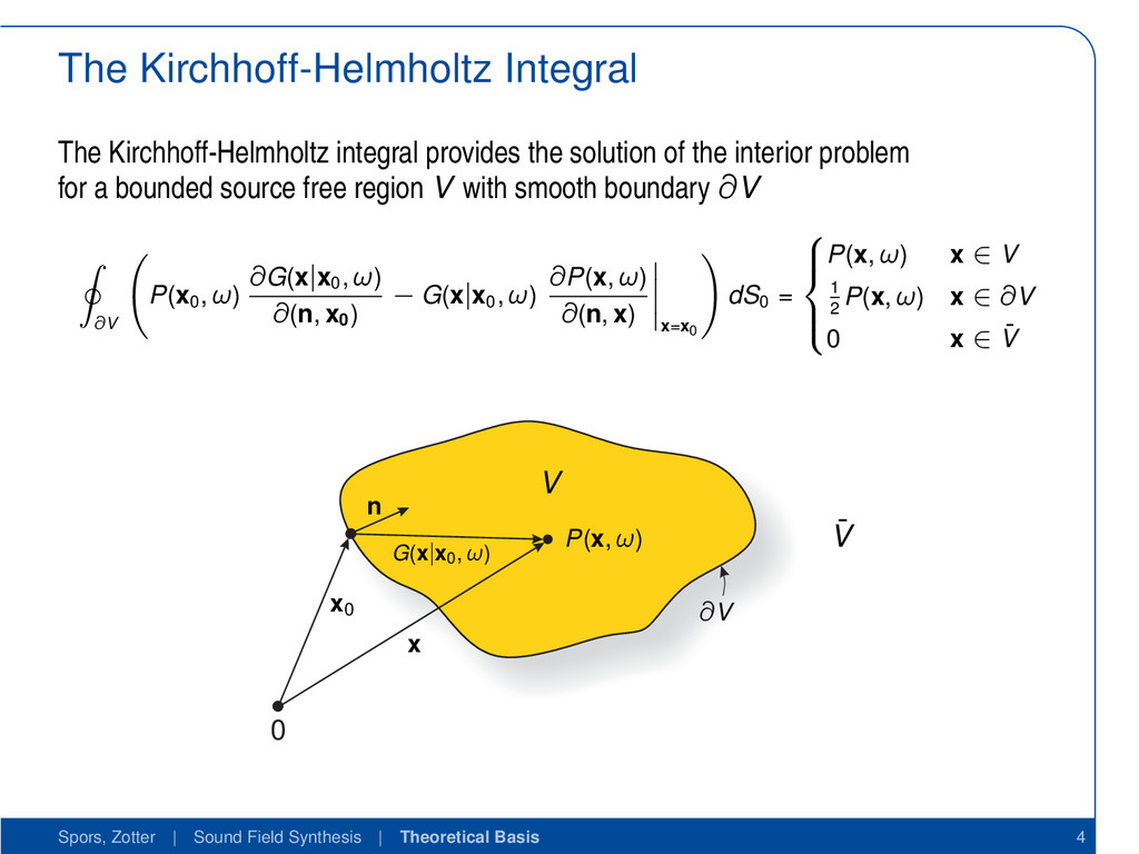
5. The Kirchhoff-Helmholtz Integral The Kirchhoff-Helmholtz integral provides the solution of the interior problem for a bounded source free region V with smooth boundary ∂V ∂V P(x0 , ω) ∂G(x|x0 , ω) ∂(n, x0 ) − G(x|x0 , ω) ∂P(x, ω) ∂(n, x) x=x0 dS0 =      P(x, ω) x ∈ V 1 2 P(x, ω) x ∈ ∂V 0 x ∈ ¯ V 0 ∂V V ¯ V n x x0 G(x|x0 , ω) P(x, ω) Spors, Zotter | Sound Field Synthesis | Theoretical Basis 4
6. The Kirchhoff-Helmholtz Integral The Kirchhoff-Helmholtz integral provides the solution of the interior problem for a bounded source free region V with smooth boundary ∂V ∂V P(x0 , ω) ∂G(x|x0 , ω) ∂(n, x0 ) − G(x|x0 , ω) ∂P(x, ω) ∂(n, x) x=x0 dS0 =      P(x, ω) x ∈ V 1 2 P(x, ω) x ∈ ∂V 0 x ∈ ¯ V Definition of the directional derivative ∂P(x, ω) ∂(n, x) x=x0 = ∇x P(x, ω), n(x) x=x0 External problem • exchange results for V and ¯ V on right hand side • reverse normal vector n or reverse signs on the right hand side Spors, Zotter | Sound Field Synthesis | Theoretical Basis 4
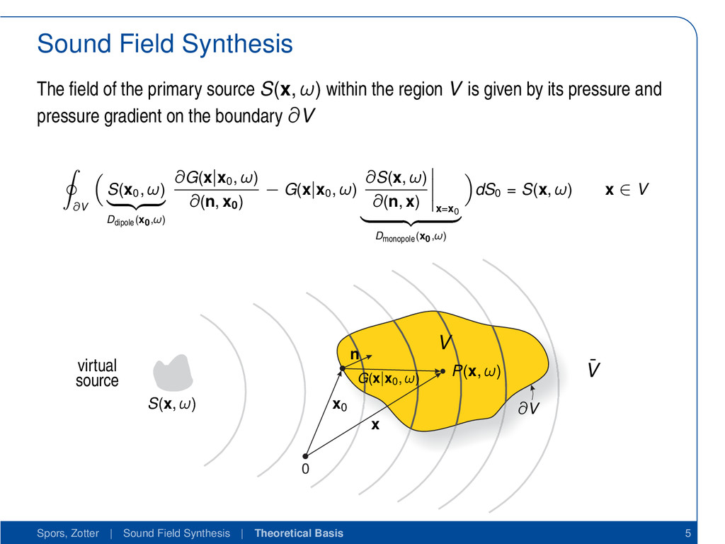
7. Sound Field Synthesis The field of the primary source S(x, ω) within the region V is given by its pressure and pressure gradient on the boundary ∂V ∂V S(x0 , ω) Ddipole(x0,ω) ∂G(x|x0 , ω) ∂(n, x0 ) − G(x|x0 , ω) ∂S(x, ω) ∂(n, x) x=x0 Dmonopole(x0,ω) dS0 = S(x, ω) x ∈ V 0 S(x, ω) ∂V V ¯ V virtual source n x x0 G(x|x0 , ω) P(x, ω) Spors, Zotter | Sound Field Synthesis | Theoretical Basis 5
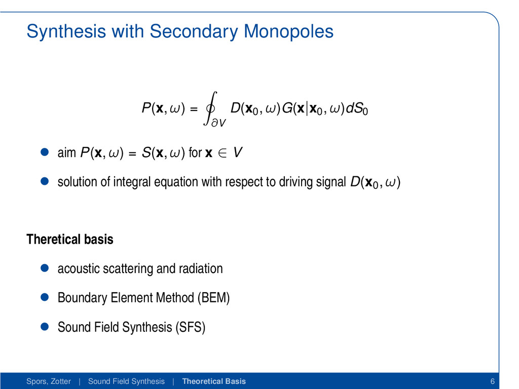
8. Synthesis with Secondary Monopoles P(x, ω) = ∂V D(x0 , ω)G(x|x0 , ω)dS0 • aim P(x, ω) = S(x, ω) for x ∈ V • solution of integral equation with respect to driving signal D(x0 , ω) Theretical basis • acoustic scattering and radiation • Boundary Element Method (BEM) • Sound Field Synthesis (SFS) Spors, Zotter | Sound Field Synthesis | Theoretical Basis 6
9. Overview – Single Layer Solutions 1. Equivalent Scattering Approach 2. explicit solution of the single layer potential 3. high-frequency approximation of the Kirchhoff-Helmholtz integral Spors, Zotter | Sound Field Synthesis | Equivalent Scattering Approach 7
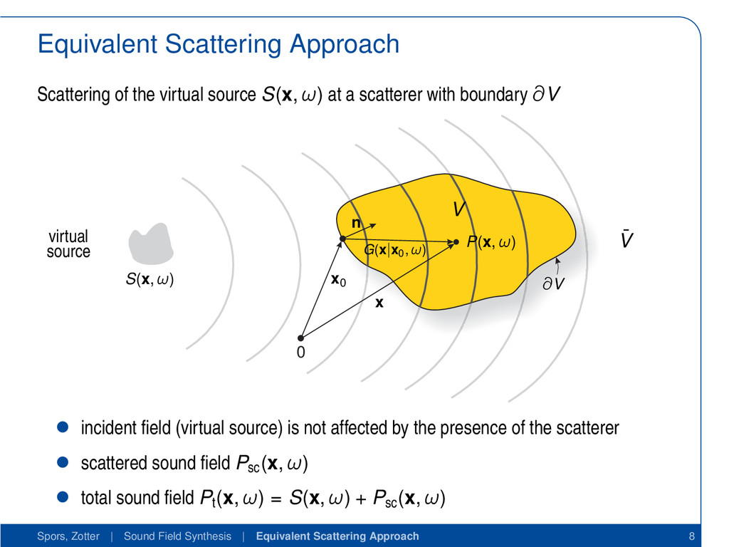
10. Equivalent Scattering Approach Scattering of the virtual source S(x, ω) at a scatterer with boundary ∂V 0 S(x, ω) ∂V V ¯ V virtual source n x x0 G(x|x0 , ω) P(x, ω) • incident field (virtual source) is not affected by the presence of the scatterer • scattered sound field Psc (x, ω) • total sound field Pt (x, ω) = S(x, ω) + Psc (x, ω) Spors, Zotter | Sound Field Synthesis | Equivalent Scattering Approach 8
11. Equivalent Scattering Approach (cont’d) The total sound field is then given as [Williams, eq.(8.37)] S(x, ω) + ∂V G(x|x0 , ω) ∂Pt (x, ω) ∂(n, x) x=x0 − Pt (x0 , ω) ∂G(x|x0 , ω) ∂(n, x0 ) dS0 =      0 x ∈ V 1 2 Pt (x, ω) x ∈ ∂V Pt (x, ω) x ∈ ¯ V Pressure release (Dirichlet) boundary ∂V ⇒ Pt (x, ω) = 0 for x ∈ ∂V ∂V G(x|x0 , ω) ∂Pt (x, ω) ∂(n, x) x=x0 −D(x0,ω) dS0 =      −S(x, ω) x ∈ V −S(x, ω) x ∈ ∂V Psc (x, ω) x ∈ ¯ V • accurate synthesis of virtual source within listening area V • driving function is given by directional derivative of total sound field Pt • requires knowledge of the scattered field Psc (x, ω) Spors, Zotter | Sound Field Synthesis | Equivalent Scattering Approach 9
12. Spherical Secondary Source Distribution Plane wave with traveling direction (βpw , αpw ) as virtual source Spw (x, ω) = 4π ∞ n=0 n m=−n (−i)njn ( ω c r)Ym n (βpw , αpw )∗Ym n (β, α) Scattering of plane wave at sphere with pressure release boundaries [Gumerov et al. 2004] Psc,pw (x, ω) = −4π ∞ n=0 n m=−n (−i)n jn (ω c R) h(2) n (ω c R) h(2) n ( ω c r)Ym n (βpw , αpw )∗Ym n (β, α) Calculation of driving function • superposition of virtual source and scattered sound field • directional derivative with inward pointing radial unit vector ⇒ Analytic (Near-Field Compensated) Higher-Order Ambisonics [Ahrens et al. 2008] Spors, Zotter | Sound Field Synthesis | Equivalent Scattering Approach 10
13. Example – Equivalent Scattering Approach Scattered sound field Psc,pw (x, ω) x (m) y (m) −3 −2 −1 0 1 2 3 −3 −2 −1 0 1 2 3 3D ESA, f = 500 Hz, βpw = 90o, αpw = 90o, R = 1.5 m, z = 0 Spors, Zotter | Sound Field Synthesis | Equivalent Scattering Approach 11
14. Example – Equivalent Scattering Approach Scattered and incident sound field Psc,pw (x, ω) + Spw (x, ω) x (m) y (m) −3 −2 −1 0 1 2 3 −3 −2 −1 0 1 2 3 3D ESA, f = 500 Hz, βpw = 90o, αpw = 90o, R = 1.5 m, z = 0 Spors, Zotter | Sound Field Synthesis | Equivalent Scattering Approach 11
15. Example – Equivalent Scattering Approach Synthesized sound field P(x, ω) x (m) y (m) −3 −2 −1 0 1 2 3 −3 −2 −1 0 1 2 3 3D ESA, f = 500 Hz, βpw = 90o, αpw = 90o, R = 1.5 m, z = 0 Spors, Zotter | Sound Field Synthesis | Equivalent Scattering Approach 11
16. Is the Solution Unique? The scattering problem could degenerate to a trivial problem if S(x, ω) = 0 for x ∈ ∂V ∂V D(x0 , ω)G(x|x0 , ω)dS0 = 0 Uniqueness of solution can be ensured by additional constraints • CHIEF point method [Schenk 1968] • Burton-Miller method [Burton et al. 1971] • define pressure on symmetry axis of rotationally symmetric problems e.g. analytic NFC-HOA [Ahrens et al. 2008] Spors, Zotter | Sound Field Synthesis | Equivalent Scattering Approach 12
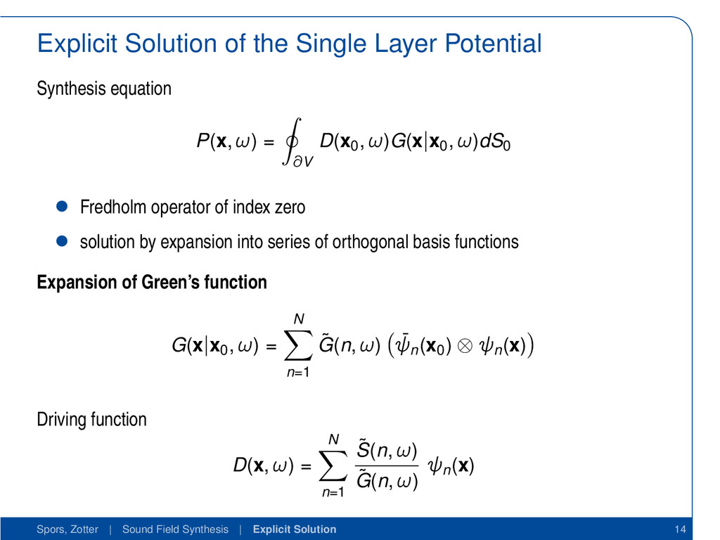
17. Overview – Single Layer Solutions 1. Equivalent Scattering Approach 2. explicit solution of the single layer potential 3. high-frequency approximation of the Kirchhoff-Helmholtz integral Spors, Zotter | Sound Field Synthesis | Explicit Solution 13
18. Explicit Solution of the Single Layer Potential Synthesis equation P(x, ω) = ∂V D(x0 , ω)G(x|x0 , ω)dS0 • Fredholm operator of index zero • solution by expansion into series of orthogonal basis functions Expansion of Green’s function G(x|x0 , ω) = N n=1 ˜ G(n, ω) ¯ ψn (x0 ) ⊗ ψn (x) Driving function D(x, ω) = N n=1 ˜ S(n, ω) ˜ G(n, ω) ψn (x) Spors, Zotter | Sound Field Synthesis | Explicit Solution 14
19. Overview – Single Layer Solutions 1. Equivalent Scattering Approach 2. explicit solution of the single layer potential 3. high-frequency approximation of the Kirchhoff-Helmholtz integral Spors, Zotter | Sound Field Synthesis | High-Frequency Approximation 15
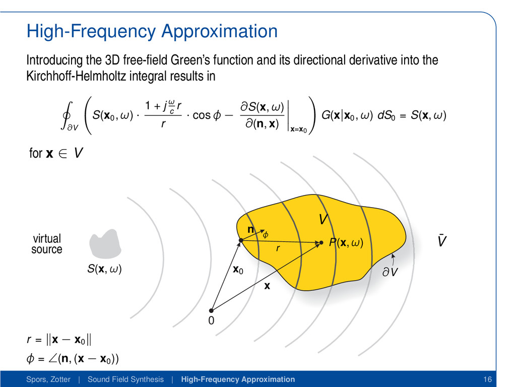
20. High-Frequency Approximation Introducing the 3D free-field Green’s function and its directional derivative into the Kirchhoff-Helmholtz integral results in ∂V S(x0 , ω) · 1 + j ω c r r · cos φ − ∂S(x, ω) ∂(n, x) x=x0 G(x|x0 , ω) dS0 = S(x, ω) for x ∈ V 0 S(x, ω) ∂V V ¯ V virtual source n x x0 r P(x, ω) φ r = x − x0 φ = ∠(n, (x − x0 )) Spors, Zotter | Sound Field Synthesis | High-Frequency Approximation 16
21. High-Frequency Approximation Introducing the 3D free-field Green’s function and its directional derivative into the Kirchhoff-Helmholtz integral results in ∂V S(x0 , ω) · 1 + j ω c r r · cos φ − ∂S(x, ω) ∂(n, x) x=x0 G(x|x0 , ω) dS0 = S(x, ω) for x ∈ V Stationary phase approximation 1. (x − x0 )||n ⇒ cos φ = 1 2. ω c r ≫ 1 ⇒ 1+j ω c r r → j ω c ∂V j ω c S(x0 , ω) − ∂S(x, ω) ∂(n, x) x=x0 D(x0,ω) G(x|x0 , ω) dS0 ≈ S(x, ω) Approximation is known as the high-frequency BEM [Herrin et al. 2003] Spors, Zotter | Sound Field Synthesis | High-Frequency Approximation 16
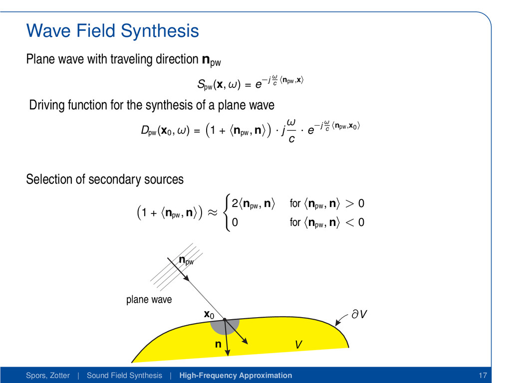
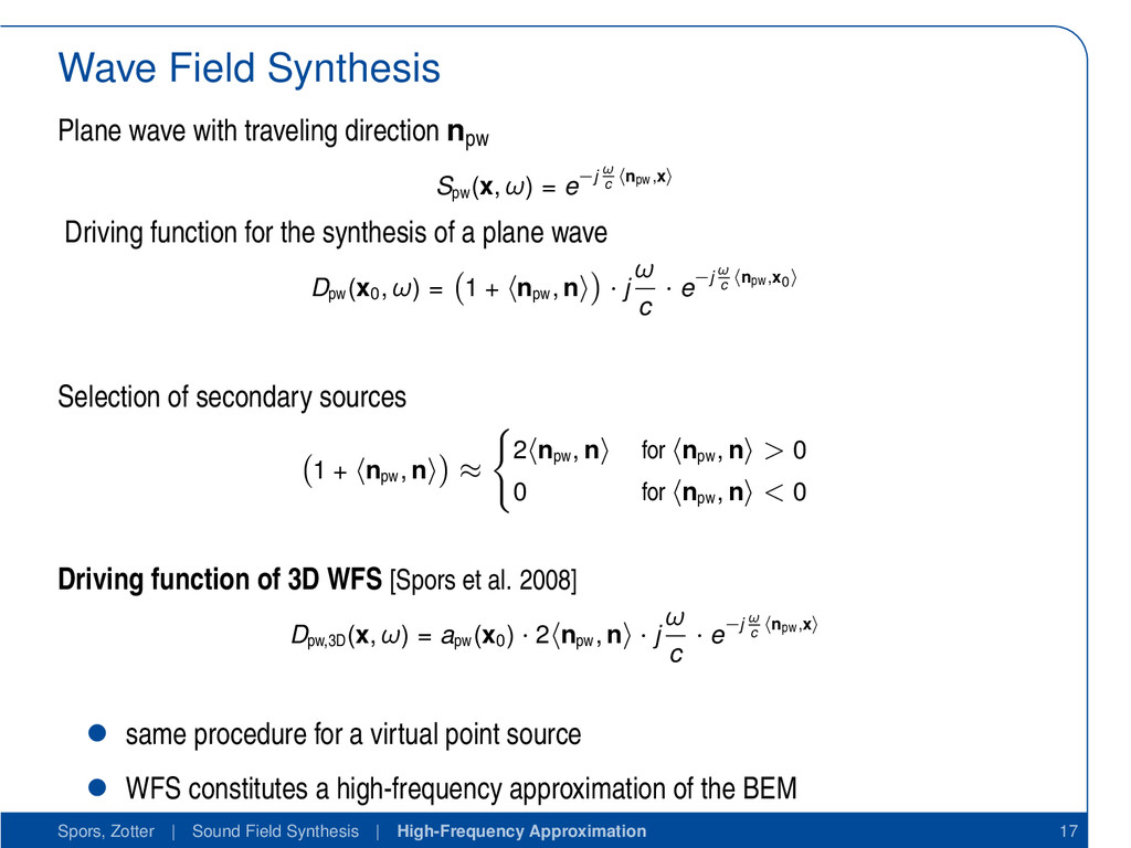
22. Wave Field Synthesis Plane wave with traveling direction npw Spw (x, ω) = e−j ω c npw,x Driving function for the synthesis of a plane wave Dpw (x0 , ω) = 1 + npw , n · j ω c · e−j ω c npw,x0 Selection of secondary sources 1 + npw , n ≈ 2 npw , n for npw , n > 0 0 for npw , n < 0 ∂V V n x0 npw plane wave Spors, Zotter | Sound Field Synthesis | High-Frequency Approximation 17
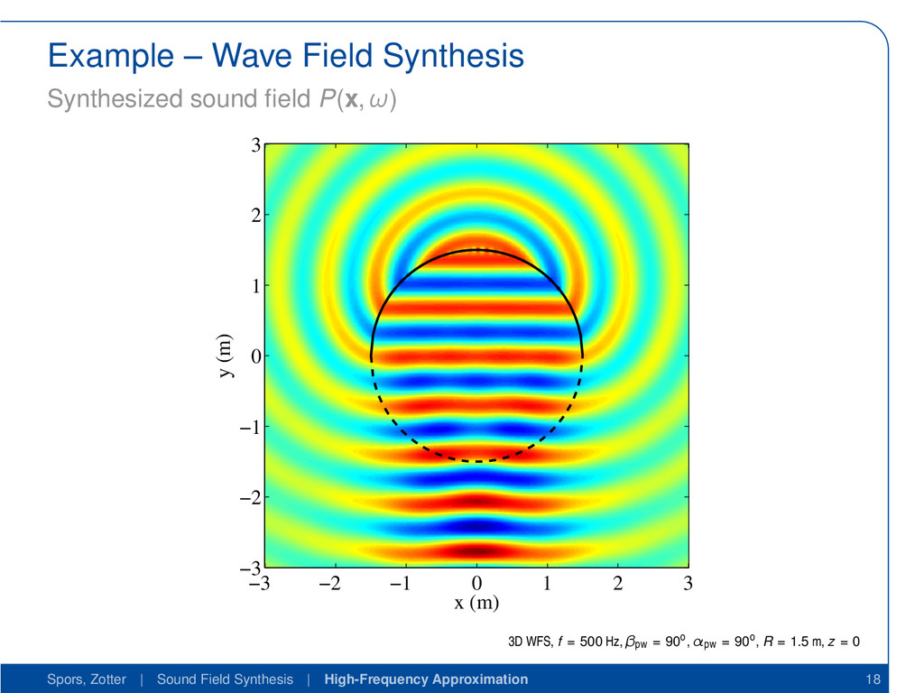
23. Wave Field Synthesis Plane wave with traveling direction npw Spw (x, ω) = e−j ω c npw,x Driving function for the synthesis of a plane wave Dpw (x0 , ω) = 1 + npw , n · j ω c · e−j ω c npw,x0 Selection of secondary sources 1 + npw , n ≈ 2 npw , n for npw , n > 0 0 for npw , n < 0 Driving function of 3D WFS [Spors et al. 2008] Dpw,3D (x, ω) = apw (x0 ) · 2 npw , n · j ω c · e−j ω c npw,x • same procedure for a virtual point source • WFS constitutes a high-frequency approximation of the BEM Spors, Zotter | Sound Field Synthesis | High-Frequency Approximation 17
24. Example – Wave Field Synthesis Synthesized sound field P(x, ω) x (m) y (m) −3 −2 −1 0 1 2 3 −3 −2 −1 0 1 2 3 3D WFS, f = 500 Hz, βpw = 90o, αpw = 90o, R = 1.5 m, z = 0 Spors, Zotter | Sound Field Synthesis | High-Frequency Approximation 18
25. Comparison of Approaches Equivalent Scattering Approach (e.g. Higher-order Ambisonics) • global dependency of driving function • analytic driving functions for regular geometries only • exact reproduction within entire listening area possible Approximation of Kirchhoff-Helmholtz Integral (e.g. Wave Field Synthesis) • local dependency of driving function • analytic driving functions for arbitrary (convex) geometries • exact reproduction only for planar systems, minor degradations for curved systems Spors, Zotter | Sound Field Synthesis | High-Frequency Approximation 19
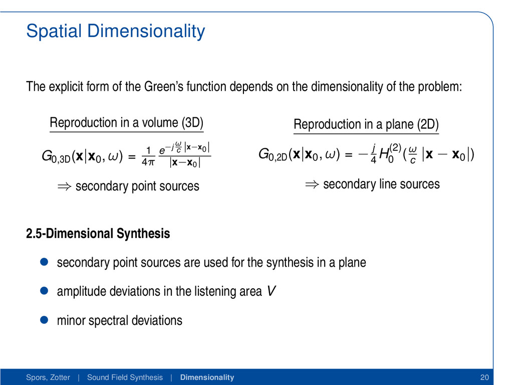
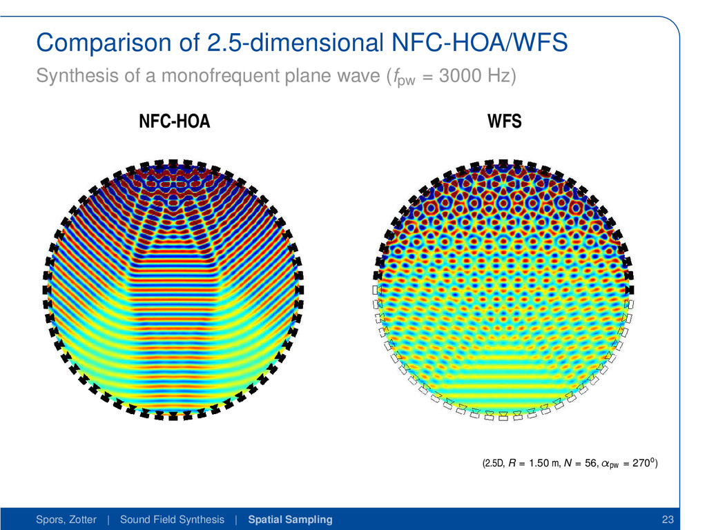
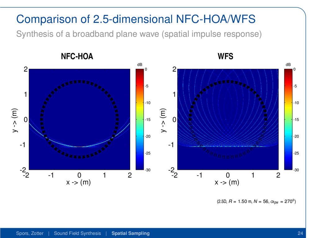
26. Spatial Dimensionality The explicit form of the Green’s function depends on the dimensionality of the problem: Reproduction in a volume (3D) G0,3D (x|x0 , ω) = 1 4π e−j ω c |x−x0 | |x−x0 | ⇒ secondary point sources Reproduction in a plane (2D) G0,2D (x|x0 , ω) = − j 4 H(2) 0 (ω c |x − x0 |) ⇒ secondary line sources 2.5-Dimensional Synthesis • secondary point sources are used for the synthesis in a plane • amplitude deviations in the listening area V • minor spectral deviations Spors, Zotter | Sound Field Synthesis | Dimensionality 20
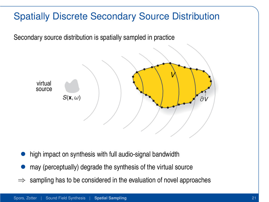
27. Spatially Discrete Secondary Source Distribution Secondary source distribution is spatially sampled in practice S(x, ω) ∂V V virtual source • high impact on synthesis with full audio-signal bandwidth • may (perceptually) degrade the synthesis of the virtual source ⇒ sampling has to be considered in the evaluation of novel approaches Spors, Zotter | Sound Field Synthesis | Spatial Sampling 21
28. Spatial Sampling of Secondary Source Distribution ˜ G0 (x, ω) D(x0 , ω) DS (x0 , ω) PS (x, ω) n ∆x spatial sampling • sampling of driving function, interpolation by secondary sources • description by spatio-temporal spectra of driving function/secondary sources • intuitive anti-aliasing condition ∆x < λ 2 does not hold in general Sampling for linear/circular/spherical boundaries [Spors et al. 2006, Ahrens et al. 2012] • repetitions (and overlap) of spatial spectrum of driving function • band-limitation of spatial spectrum improves sampling artifacts (e.g. HOA) Spors, Zotter | Sound Field Synthesis | Spatial Sampling 22
29. Comparison of 2.5-dimensional NFC-HOA/WFS Synthesis of a monofrequent plane wave (fpw = 500 Hz) NFC-HOA WFS (2.5D, R = 1.50 m, N = 56, αpw = 270o) Spors, Zotter | Sound Field Synthesis | Spatial Sampling 23
30. Comparison of 2.5-dimensional NFC-HOA/WFS Synthesis of a monofrequent plane wave (fpw = 3000 Hz) NFC-HOA WFS (2.5D, R = 1.50 m, N = 56, αpw = 270o) Spors, Zotter | Sound Field Synthesis | Spatial Sampling 23
31. Comparison of 2.5-dimensional NFC-HOA/WFS Synthesis of a broadband plane wave (spatial impulse response) NFC-HOA x -> (m) y -> (m) -2 -1 0 1 2 -2 -1 0 1 2 dB -30 -25 -20 -15 -10 -5 0 WFS x -> (m) y -> (m) -2 -1 0 1 2 -2 -1 0 1 2 dB -30 -25 -20 -15 -10 -5 0 (2.5D, R = 1.50 m, N = 56, αpw = 270o) Spors, Zotter | Sound Field Synthesis | Spatial Sampling 24
32. Comparison of 2.5-dimensional NFC-HOA/WFS Synthesis of a broadband plane wave (spatial impulse response) NFC-HOA x -> (m) y -> (m) -2 -1 0 1 2 -2 -1 0 1 2 dB -30 -25 -20 -15 -10 -5 0 WFS x -> (m) y -> (m) -2 -1 0 1 2 -2 -1 0 1 2 dB -30 -25 -20 -15 -10 -5 0 (2.5D, R = 1.50 m, N = 56, αpw = 270o) Spors, Zotter | Sound Field Synthesis | Spatial Sampling 24
33. Comparison of 2.5-dimensional NFC-HOA/WFS Synthesis of a broadband plane wave (spatial impulse response) NFC-HOA x -> (m) y -> (m) -2 -1 0 1 2 -2 -1 0 1 2 dB -30 -25 -20 -15 -10 -5 0 WFS x -> (m) y -> (m) -2 -1 0 1 2 -2 -1 0 1 2 dB -30 -25 -20 -15 -10 -5 0 (2.5D, R = 1.50 m, N = 56, αpw = 270o) Spors, Zotter | Sound Field Synthesis | Spatial Sampling 24
34. Conclusions • theory of sound field synthesis is well grounded • spatial sampling reduces achievable accuracy considerably • monochromatic sound fields are not sufficient for evaluation • perception of synthetic sound fields plays an inportant role Reproducible Reserach • software implementations have high impact on results • Sound Field Synthesis (SFS) Toolbox http://github.com/sfstoolbox • SoundScape Renderer (SSR) http://www.spatialaudio.net/ssr Spors, Zotter | Sound Field Synthesis | Conclusions 25
35. Thanks for your attention! www.spatialaudio.net
36. Simple Source Formulation [Williams] Interior Problem (n points inward) ∂V S(x0 , ω) ∂G(x|x0 , ω) ∂(n, x0 ) − G(x|x0 , ω) ∂S(x, ω) ∂(n, x) x=x0 dS0 =      S(x, ω) x ∈ V 1 2 S(x, ω) x ∈ ∂V 0 x ∈ ¯ V Exterior Problem (n points inward) ∂V Psc (x0 , ω) ∂G(x|x0 , ω) ∂(n, x0 ) − G(x|x0 , ω) ∂Psc (x, ω) ∂(n, x) x=x0 dS0 =      0 x ∈ V −1 2 Psc (x, ω) x ∈ ∂V −Psc x ∈ ¯ V (Interior)+(Exterior) together with S(x, ω) + Psc (x, ω) = 0 for x ∈ ∂V − ∂V G(x|x0 , ω) ∂(S(x, ω) + Psc (x, ω) ∂(n, x) x=x0 dS0 =      S(x, ω) x ∈ V S(x, ω) x ∈ ∂V −Psc (x, ω) x ∈ ¯ V Spors, Zotter | Sound Field Synthesis | Conclusions 26