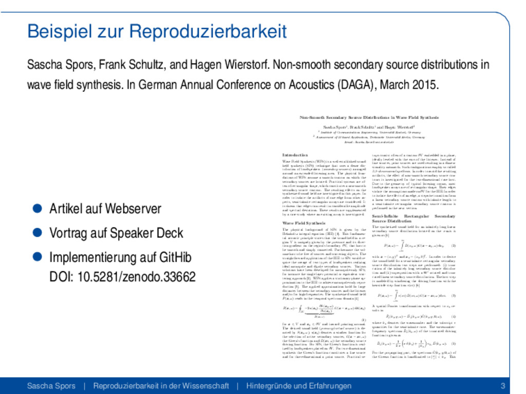
Non-smooth secondary source distributions in wave field synthesis. In German Annual Conference on Acoustics (DAGA), March 2015. Artikel auf Webserver Vortrag auf Speaker Deck Implementierung auf GitHib DOI: 10.5281/zenodo.33662 Non-Smooth Secondary Source Distributions in Wave Field Synthesis Sascha Spors1, Frank Schultz1 and Hagen Wierstorf2 1 Institute of Communications Engineering, Universit¨ at Rostock, Germany 2 Assessement of IP-based Applications, Technische Universit¨ at Berlin, Germany Email:
[email protected] Introduction Wave Field Synthesis (WFS) is a well-established sound field synthesis (SFS) technique that uses a dense dis- tribution of loudspeakers (secondary sources) arranged around an extended listening area. The physical foun- dations of WFS assume a smooth contour on which the secondary sources are located. Practical systems are of- ten of rectangular shape, which constitutes a non-smooth secondary source contour. The resulting effects on the synthesized sound field are investigated in this paper. In order to isolate the artifacts of one edge from other as- pects, semi-infinite rectangular arrays are considered. It is shown that edges can result in considerable amplitude and spectral deviations. These results are supplemented by a case-study where an existing array is investigated. Wave Field Synthesis The physical background of SFS is given by the Helmholtz integral equation (HIE) [1]. This fundamen- tal acoustic principle states that the sound field in a re- gion V is uniquely given by the pressure and its direc- tion gradient on the region’s boundary ∂V , that has to be smooth and simply connected. Furthermore the vol- ume has to be free of sources and scattering objects. The straightforward application of the HIE to SFS would re- quire the useage of two types of loudspeakers realizing ideal monopole and dipole secondary sources. Various solutions have been developed for monopole-only SFS, for instance the single layer potential or equivalent scat- tering approach [2]. WFS applies a stationary-phase ap- proximation to the HIE to achieve monopole-only repro- duction [3]. The applied approximations hold for large distances between the secondary sources and the listener and/or for high-frequencies. The synthesized sound field P(x, ω) reads in the temporal spectrum domain [4] P(x, ω) = ∂V −2 a(x0 ) ∂S(x0 , ω) ∂n(x0 ) D(x0,ω) G(x − x0 , ω) dA(x0 ) (1) for x ∈ V and x0 ∈ ∂V and inward pointing normal. The desired sound field (primary/virtual source) is de- noted by S(x0 , ω), a(x0 ) denotes a window function for the selection of active secondary sources, G(x − x0 , ω) the Green’s function and D(x0 , ω) the secondary source driving function. For SFS, the Green’s function is real- ized by loudspeakers placed on ∂V . For two-dimensional synthesis the Green’s function constitutes a line source and for three-dimensional a point source. Practical se- tups consist often of a contour ∂V embedded in a plane, ideally leveled with the ears of the listener. Instead of line sources, point sources are used resulting in a dimen- sionality mismatch. Such configurations employ so called 2.5-dimensional synthesis. In order to avoid the resulting artifacts, the effect of non-smooth secondary source con- tours is investigated for the two-dimensional case first. Due to the geometry of typical listening rooms, most loudspeaker arrays are of rectangular shape. Their edges violate the assumptions made on ∂V for the HIE. In order to isolate the effects of an edge, a stepwise transition from a linear secondary source contour with infinite length to a semi-infinite rectangular secondary source contour is performed in the next section. Semi-Infinite Rectangular Secondary Source Distribution The synthesized sound field for an infinitely long linear secondary source distribution located on the x-axis is given as [5] P(x, ω) = ∞ −∞ D(x0 , ω) G(x − x0 , ω) dx0 , (2) with x = (x, y)T and x0 = (x0 , 0)T . In order to derive the sound field for a semi-infinite rectangular secondary source distribution two steps are performed: (i) trun- cation of the infinitely long secondary source distribu- tion and (ii) superposition with a 90◦ rotated and trun- cated linear secondary source distribution. The first step is modeled by windowing the driving function with the heaviside step function (x0 ) [6] P(x, ω) = ∞ −∞ (x0 ) D(x0 , ω) G(x − x0 , ω) dx0 . (3) A spatial Fourier transformation with respect to x0 re- sults in ˜ P (kx , y, ω) = ˜ D (kx , ω) ˜ G(kx , y, 0, ω), (4) where kx denotes the wavenumber and the subscript quantities for the semi-infinite case. The wavenumber- frequency spectrum ˜ D (kx , ω) of the truncated driving function is given as ˜ D (kx , ω) = 1 2 π π δ(kx ) + 1 j kx ∗kx ˜ D(kx , ω). (5) For the propagating part, the spectrum ˜ G(kx , y, 0, ω) of the Greens function is bandlimited to |ω c | < kx . This Sascha Spors | Reproduzierbarkeit in der Wissenschaft | Hintergründe und Erfahrungen 3
![Reproduzierbarkeit Einteilung der Reproduzierbarkeit [Stodden, 2013] Empirisch Mathematisch/Technisch (’Computational’) Mathematik,](https://files.speakerdeck.com/presentations/4a2e5e9c88a249ab912c162553371c4a/slide_6.jpg)