it Related to Numerical Acoustics? Franz Zotter 1 and Sascha Spors 2 1University of Music and Performing Arts, Institute of Electronic Music and Acoustics 2Universität Rostock, Institute of Communications Engineering AES 52nd International Conference Guildford, UK
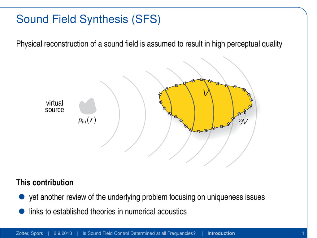
is assumed to result in high perceptual quality pin(r) ∂V V virtual source This contribution yet another review of the underlying problem focusing on uniqueness issues links to established theories in numerical acoustics Zotter, Spors | 2.9.2013 | Is Sound Field Control Determined at all Frequencies? | Introduction 1
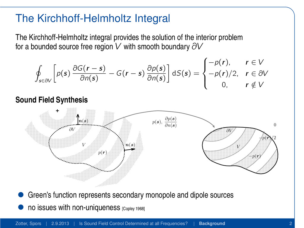
the interior problem for a bounded source free region V with smooth boundary ∂V s∈∂V p(s) ∂G(r − s) ∂n(s) − G(r − s) ∂p(s) ∂n(s) dS(s) = −p(r), r ∈ V −p(r)/2, r ∈ ∂V 0, r / ∈ V Sound Field Synthesis V V n(s) n(s) p(s), ∂p(s) ∂n(s) ∂V ∂V p(r) −p(r) −p(r)/2 0 Green’s function represents secondary monopole and dipole sources no issues with non-uniqueness [Copley 1968] Zotter, Spors | 2.9.2013 | Is Sound Field Control Determined at all Frequencies? | Background 2
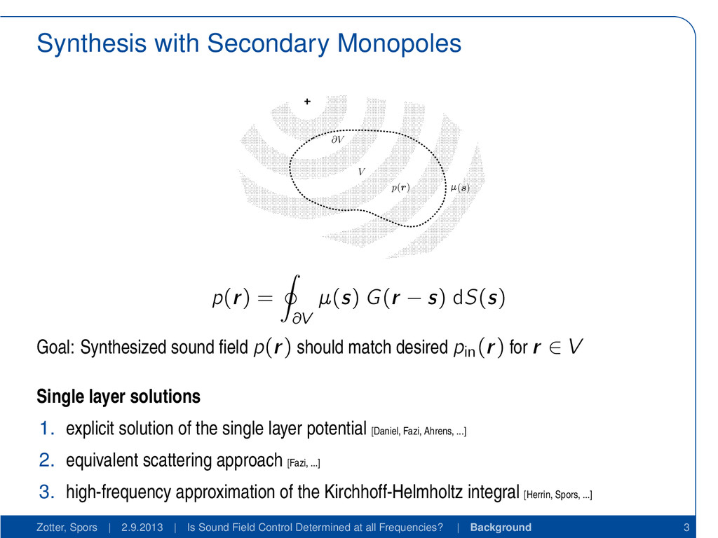
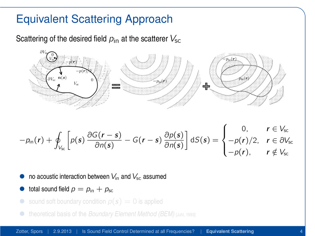
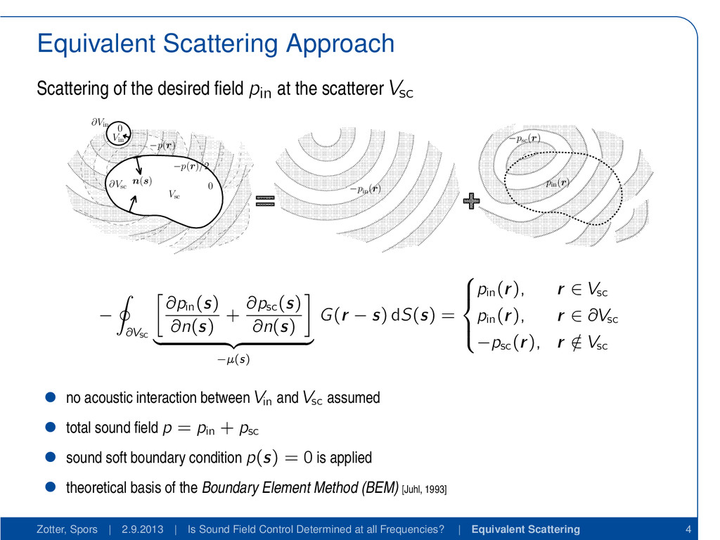
= ∂V µ(s) G(r − s) dS(s) Goal: Synthesized sound field p(r) should match desired pin(r) for r ∈ V Single layer solutions 1. explicit solution of the single layer potential [Daniel, Fazi, Ahrens, ...] 2. equivalent scattering approach [Fazi, ...] 3. high-frequency approximation of the Kirchhoff-Helmholtz integral [Herrin, Spors, ...] Zotter, Spors | 2.9.2013 | Is Sound Field Control Determined at all Frequencies? | Background 3
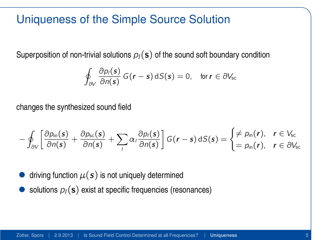
pl (s) of the sound soft boundary condition ∂V ∂pl (s) ∂n(s) G(r − s) dS(s) = 0, for r ∈ ∂Vsc changes the synthesized sound field − ∂V ∂pin (s) ∂n(s) + ∂psc (s) ∂n(s) + l αl ∂pl (s) ∂n(s) G(r − s) dS(s) = = pin (r), r ∈ Vsc = pin (r), r ∈ ∂Vsc driving function µ(s) is not uniquely determined solutions pl (s) exist at specific frequencies (resonances) Zotter, Spors | 2.9.2013 | Is Sound Field Control Determined at all Frequencies? | Uniqueness 5
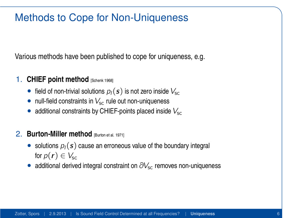
to cope for uniqueness, e.g. 1. CHIEF point method [Schenk 1968] field of non-trivial solutions pl (s) is not zero inside Vsc null-field constraints in Vsc rule out non-uniqueness additional constraints by CHIEF-points placed inside Vsc 2. Burton-Miller method [Burton et al. 1971] solutions pl (s) cause an erroneous value of the boundary integral for p(r) ∈ Vsc additional derived integral constraint on ∂Vsc removes non-uniqueness Zotter, Spors | 2.9.2013 | Is Sound Field Control Determined at all Frequencies? | Uniqueness 6
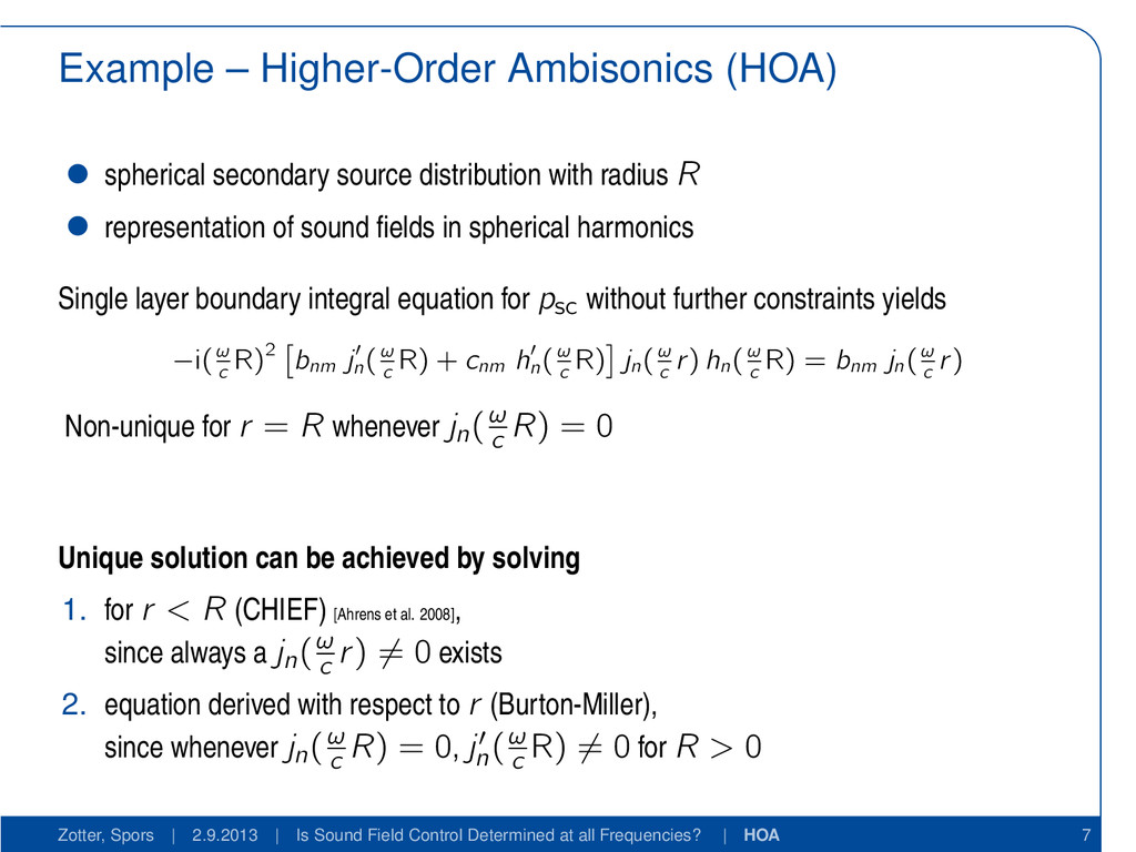
radius R representation of sound fields in spherical harmonics Single layer boundary integral equation for psc without further constraints yields −i(ω c R)2 bnm j′ n (ω c R) + cnm h′ n (ω c R) jn(ω c r) hn(ω c R) = bnm jn(ω c r) Non-unique for r = R whenever jn(ω c R) = 0 Unique solution can be achieved by solving 1. for r < R (CHIEF) [Ahrens et al. 2008] , since always a jn(ω c r) = 0 exists 2. equation derived with respect to r (Burton-Miller), since whenever jn(ω c R) = 0, j′ n (ω c R) = 0 for R > 0 Zotter, Spors | 2.9.2013 | Is Sound Field Control Determined at all Frequencies? | HOA 7
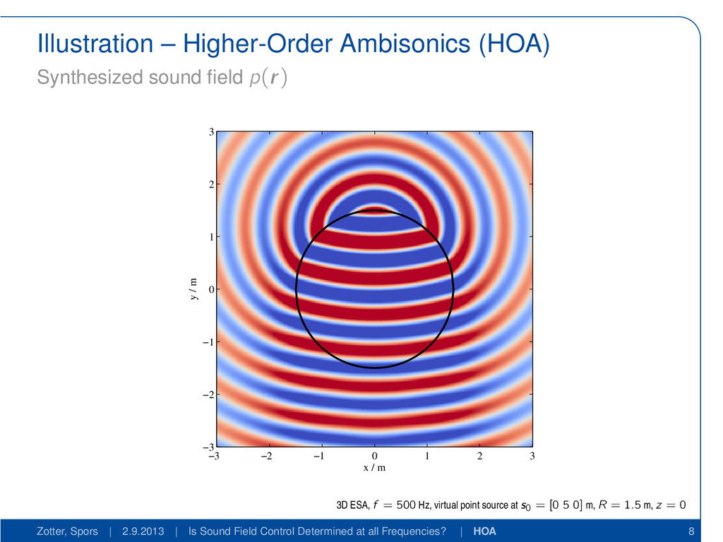
/ m y / m −3 −2 −1 0 1 2 3 −3 −2 −1 0 1 2 3 3D ESA, f = 500 Hz, virtual point source at s0 = [0 5 0] m, R = 1.5 m, z = 0 Zotter, Spors | 2.9.2013 | Is Sound Field Control Determined at all Frequencies? | HOA 8
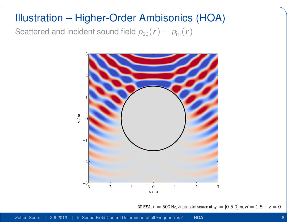
psc(r) + pin(r) x / m y / m −3 −2 −1 0 1 2 3 −3 −2 −1 0 1 2 3 3D ESA, f = 500 Hz, virtual point source at s0 = [0 5 0] m, R = 1.5 m, z = 0 Zotter, Spors | 2.9.2013 | Is Sound Field Control Determined at all Frequencies? | HOA 8
/ m y / m −3 −2 −1 0 1 2 3 −3 −2 −1 0 1 2 3 3D ESA, f = 500 Hz, virtual point source at s0 = [0 5 0] m, R = 1.5 m, z = 0 Zotter, Spors | 2.9.2013 | Is Sound Field Control Determined at all Frequencies? | HOA 8
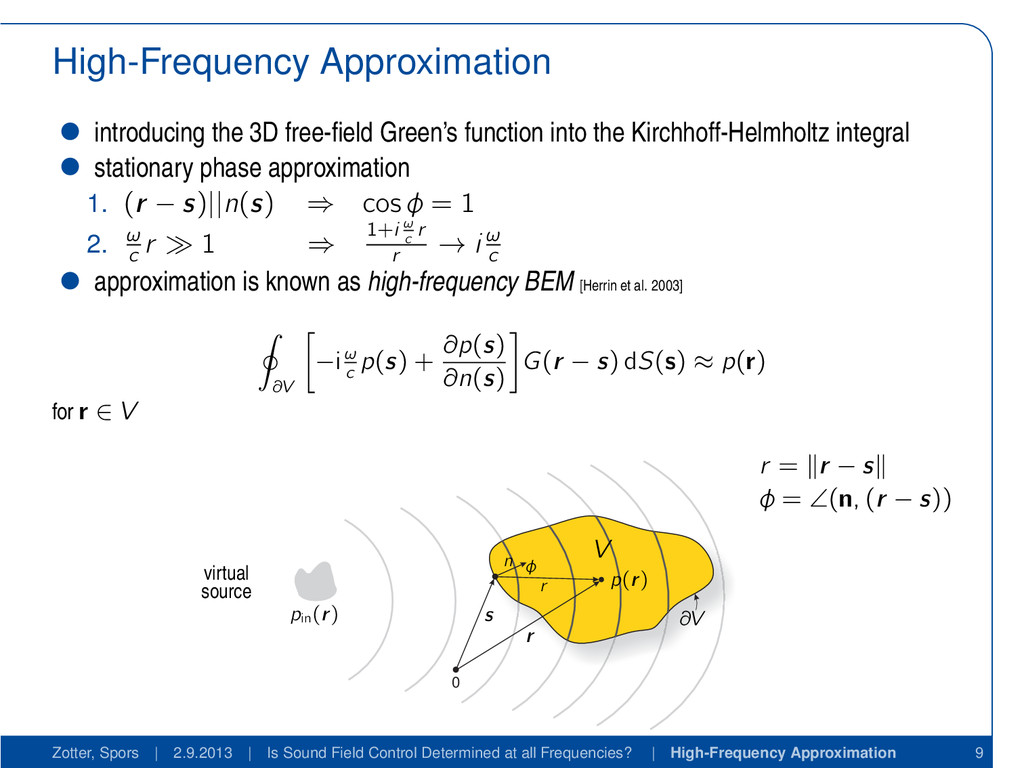
Kirchhoff-Helmholtz integral stationary phase approximation 1. (r − s)||n(s) ⇒ cos φ = 1 2. ω c r ≫ 1 ⇒ 1+i ω c r r → i ω c approximation is known as high-frequency BEM [Herrin et al. 2003] ∂V p(s) cos φ 1 + iω c r r + ∂p(s) ∂n(s) G(r − s) dS(s) = p(r) for r ∈ V 0 pin (r) ∂V V virtual source n r s r p(r) φ r = r − s φ = ∠(n, (r − s)) Zotter, Spors | 2.9.2013 | Is Sound Field Control Determined at all Frequencies? | High-Frequency Approximation 9
Kirchhoff-Helmholtz integral stationary phase approximation 1. (r − s)||n(s) ⇒ cos φ = 1 2. ω c r ≫ 1 ⇒ 1+i ω c r r → i ω c approximation is known as high-frequency BEM [Herrin et al. 2003] ∂V −iω c p(s) + ∂p(s) ∂n(s) G(r − s) dS(s) ≈ p(r) for r ∈ V 0 pin (r) ∂V V virtual source n r s r p(r) φ r = r − s φ = ∠(n, (r − s)) Zotter, Spors | 2.9.2013 | Is Sound Field Control Determined at all Frequencies? | High-Frequency Approximation 9
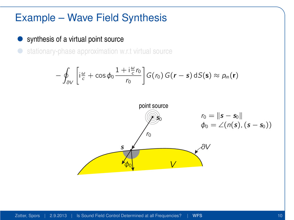
source stationary-phase approximation w.r.t virtual source − ∂V iω c + cos φ0 1 + iω c r0 r0 G(r0 ) G(r − s) dS(s) ≈ pin (r) ∂V V φ0 s s0 r0 point source r0 = s − s0 φ0 = ∠(n(s), (s − s0 )) Zotter, Spors | 2.9.2013 | Is Sound Field Control Determined at all Frequencies? | WFS 10
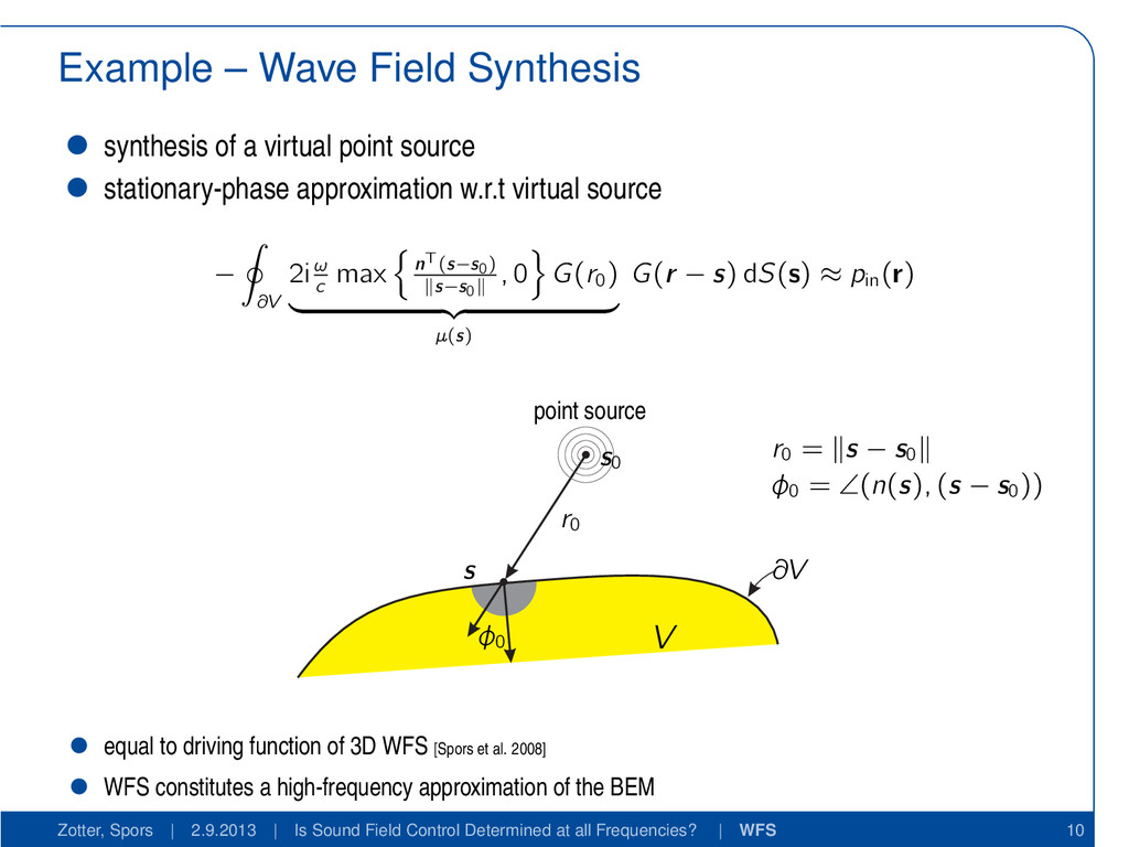
source stationary-phase approximation w.r.t virtual source − ∂V 2iω c max nT(s−s0) s−s0 , 0 G(r0 ) µ(s) G(r − s) dS(s) ≈ pin (r) ∂V V φ0 s s0 r0 point source r0 = s − s0 φ0 = ∠(n(s), (s − s0 )) equal to driving function of 3D WFS [Spors et al. 2008] WFS constitutes a high-frequency approximation of the BEM Zotter, Spors | 2.9.2013 | Is Sound Field Control Determined at all Frequencies? | WFS 10
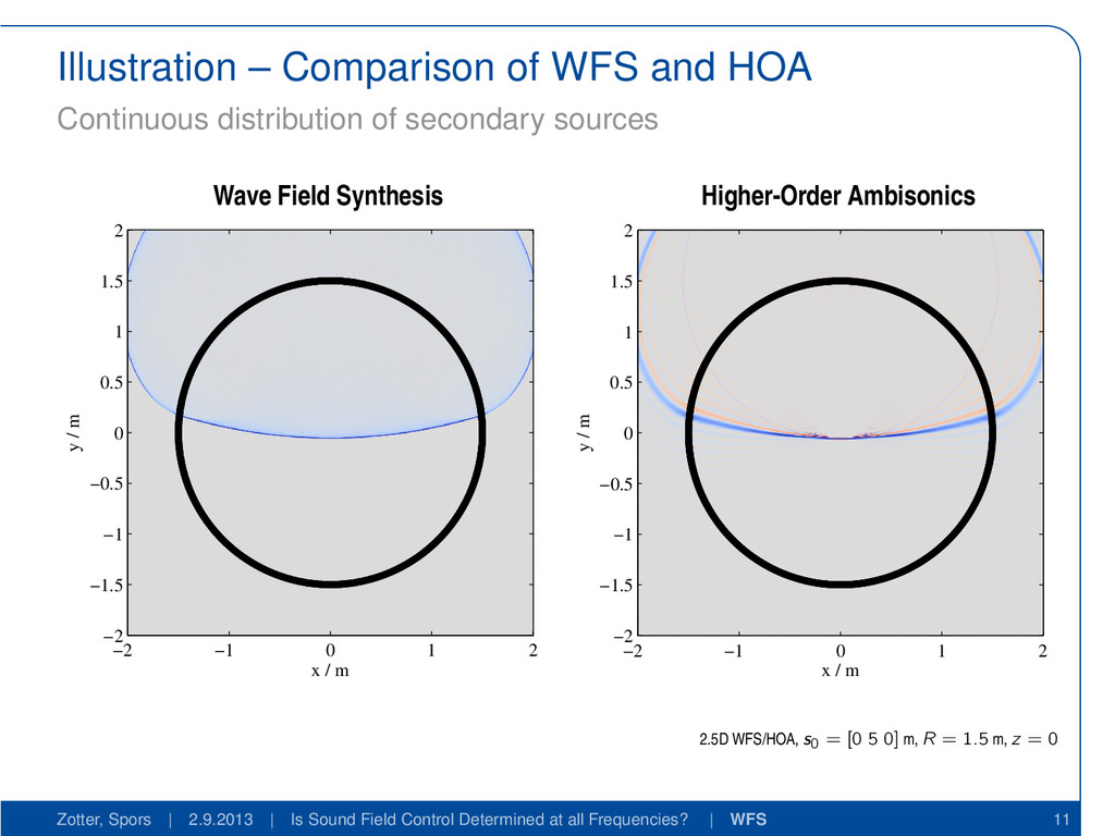
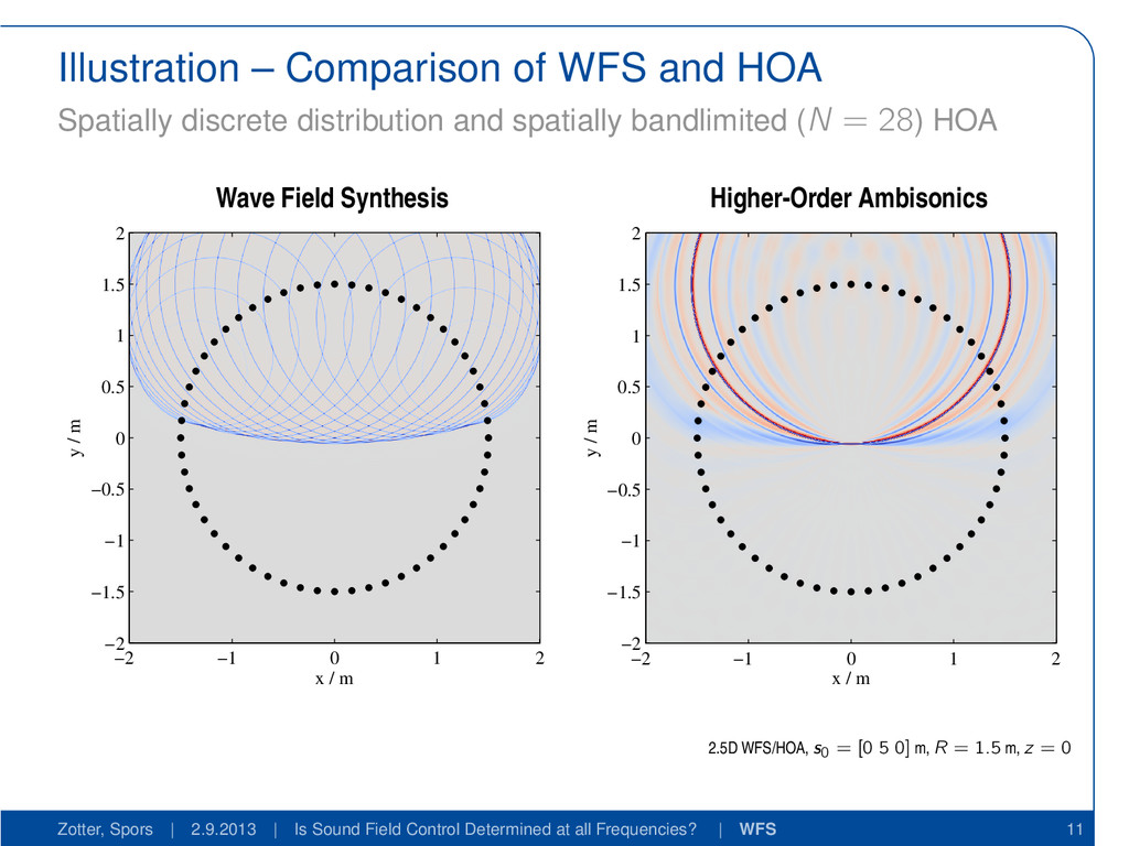
secondary sources Wave Field Synthesis x / m y / m −2 −1 0 1 2 −2 −1.5 −1 −0.5 0 0.5 1 1.5 2 Higher-Order Ambisonics x / m y / m −2 −1 0 1 2 −2 −1.5 −1 −0.5 0 0.5 1 1.5 2 2.5D WFS/HOA, s0 = [0 5 0] m, R = 1.5 m, z = 0 Zotter, Spors | 2.9.2013 | Is Sound Field Control Determined at all Frequencies? | WFS 11
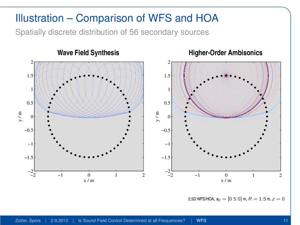
of 56 secondary sources Wave Field Synthesis x / m y / m −2 −1 0 1 2 −2 −1.5 −1 −0.5 0 0.5 1 1.5 2 Higher-Order Ambisonics x / m y / m −2 −1 0 1 2 −2 −1.5 −1 −0.5 0 0.5 1 1.5 2 2.5D WFS/HOA, s0 = [0 5 0] m, R = 1.5 m, z = 0 Zotter, Spors | 2.9.2013 | Is Sound Field Control Determined at all Frequencies? | WFS 11
and spatially bandlimited (N = 28) HOA Wave Field Synthesis x / m y / m −2 −1 0 1 2 −2 −1.5 −1 −0.5 0 0.5 1 1.5 2 Higher-Order Ambisonics x / m y / m −2 −1 0 1 2 −2 −1.5 −1 −0.5 0 0.5 1 1.5 2 2.5D WFS/HOA, s0 = [0 5 0] m, R = 1.5 m, z = 0 Zotter, Spors | 2.9.2013 | Is Sound Field Control Determined at all Frequencies? | WFS 11
sampling spatial bandlimitation directivity of loudspeakers frequency response of loudspeakers diffraction/reflections by loudspeakers listening room acoustics artifacts of 2.5-dimensional synthesis These practical artifacts have a major impact on the perceived quality! Zotter, Spors | 2.9.2013 | Is Sound Field Control Determined at all Frequencies? | Conclusion 12
uniqueness of equivalent scattering approach can be ensured WFS is a reasonable approximation with benefits (uniqueness, geometry) influence of practical constraints not well researched Thanks for your attention! www.spatialaudio.net Zotter, Spors | 2.9.2013 | Is Sound Field Control Determined at all Frequencies? | Conclusion 13