Building a Python Workflow for California Rice Monitoring From Satellite Indicators to Yield and Production

Transcript

1. Building a Python Workflow for California Rice Monitoring From Satellite Indicators to Yield and Production Takeo Shibata 0
2. - Born and raised in Aichi, Japan - Background in Geophysics - Over 30 years of experience in software and information systems - Currently working on data science and AI-related projects - Based in Southern California Areas of Interest - GIS & Remote Sensing - GeoAI / Machine Learning - Earth Observation & Satellite Data - Python for Geospatial Analysis - Open Data & Open Source GIS - Environmental, agricultural, and disaster-related applications Outside of GIS - Hiking & camping - Cycling - Train travel - Robotics & electronics projects @takeofuture dev.to/takeofuture www.linkedin.com/in/takeofuture/
3. OUTLINE ▪ ▪ ▪ ▪ ▪ ▪ ▪ ▪ ▪ ▪ ▪ ▪ ▪ ▪ Why California Rice? — and Why Sacramento? Data Sources and Processing Workflow Annual Rice Footprints with CDL Rice Area and USDA NASS Statistics Satellite and Climate Indicators Seasonal vs. Monthly Yield Signals Exploratory Climate-Stress Score Machine-Learning Design Yield Prediction Production Prediction Two Roles for Satellite and Open Data Takeaways and Next Steps References Appendices
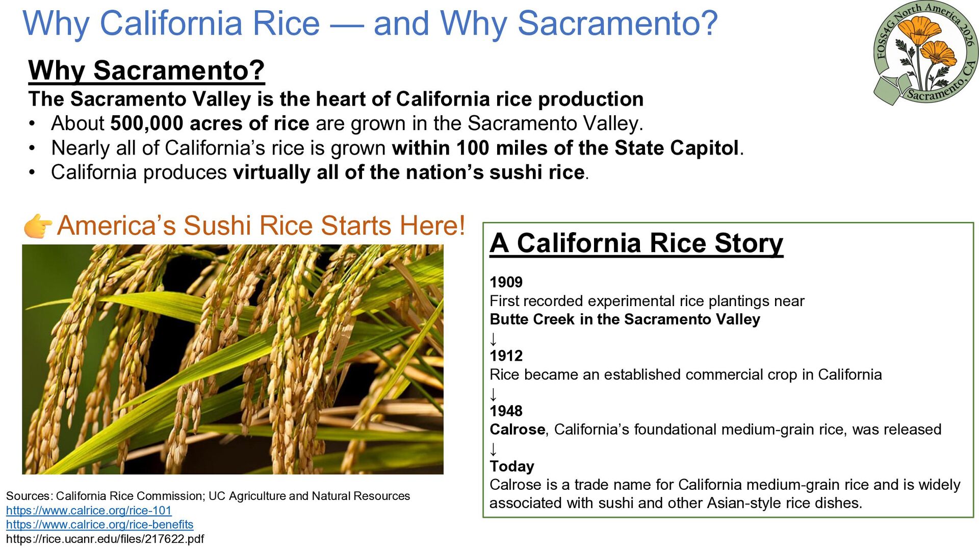
4. Why California Rice — and Why Sacramento? Why Sacramento? The Sacramento Valley is the heart of California rice production • About 500,000 acres of rice are grown in the Sacramento Valley. • Nearly all of California’s rice is grown within 100 miles of the State Capitol. • California produces virtually all of the nation’s sushi rice. America’s Sushi Rice Starts Here! Sources: California Rice Commission; UC Agriculture and Natural Resources https://www.calrice.org/rice-101 https://www.calrice.org/rice-benefits https://rice.ucanr.edu/files/217622.pdf A California Rice Story 1909 First recorded experimental rice plantings near Butte Creek in the Sacramento Valley ↓ 1912 Rice became an established commercial crop in California ↓ 1948 Calrose, California’s foundational medium-grain rice, was released ↓ Today Calrose is a trade name for California medium-grain rice and is widely associated with sushi and other Asian-style rice dishes.
5. Data Sources and Processing Workflow Processing environment: AWS EC2 · Python · GDAL/Rasterio · NumPy/Pandas → Google Colab · SciPy · scikit-learn
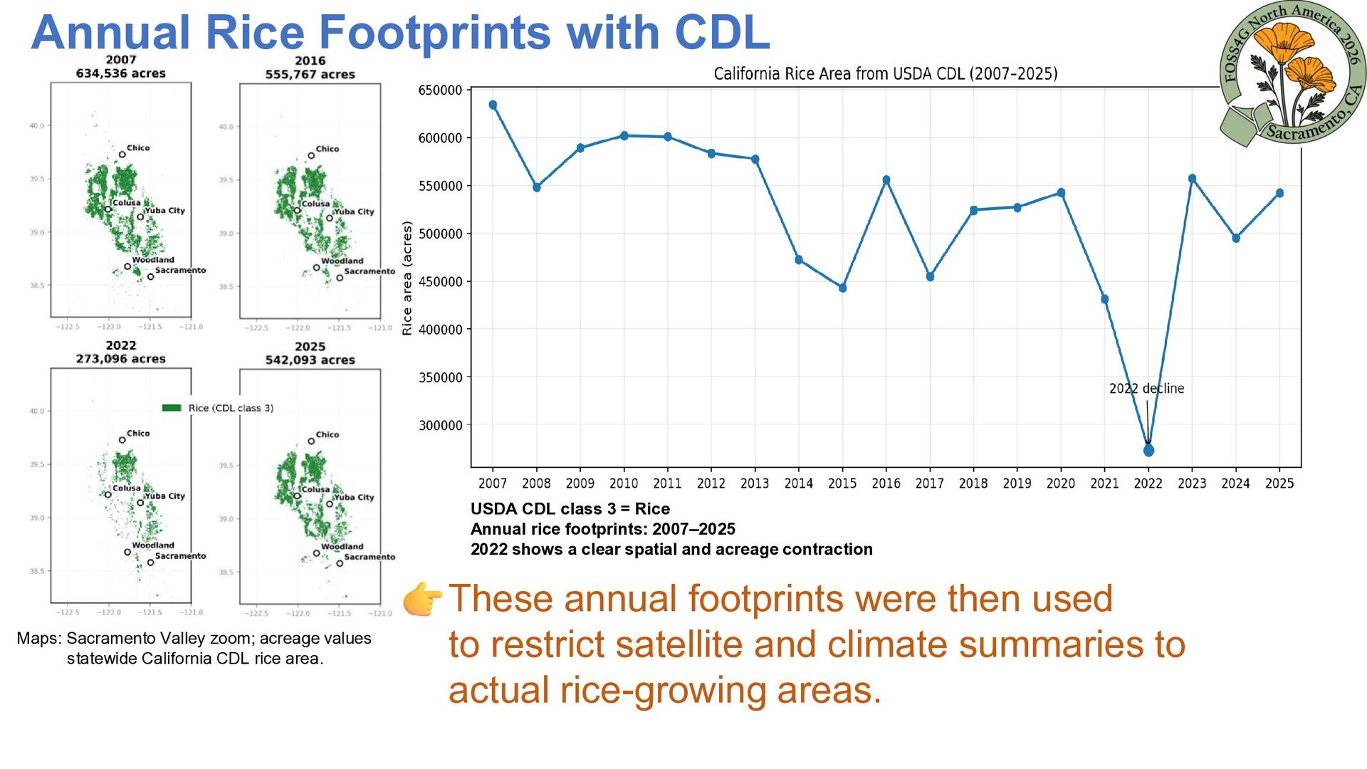
6. Annual Rice Footprints with CDL USDA CDL class 3 = Rice Annual rice footprints: 2007–2025 2022 shows a clear spatial and acreage contraction Maps: Sacramento Valley zoom; acreage values statewide California CDL rice area. These annual footprints were then used to restrict satellite and climate summaries to actual rice-growing areas.
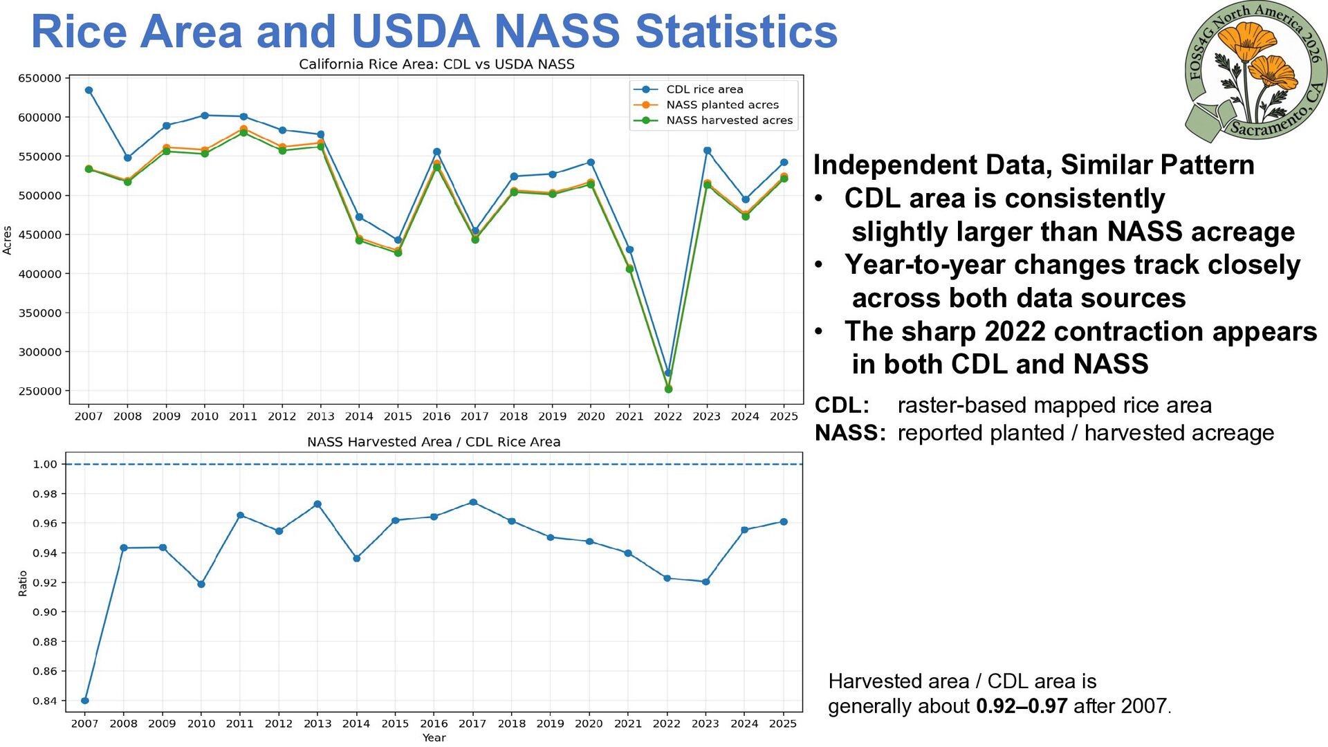
7. Rice Area and USDA NASS Statistics Independent Data, Similar Pattern • CDL area is consistently slightly larger than NASS acreage • Year-to-year changes track closely across both data sources • The sharp 2022 contraction appears in both CDL and NASS CDL: raster-based mapped rice area NASS: reported planted / harvested acreage Harvested area / CDL area is generally about 0.92–0.97 after 2007.
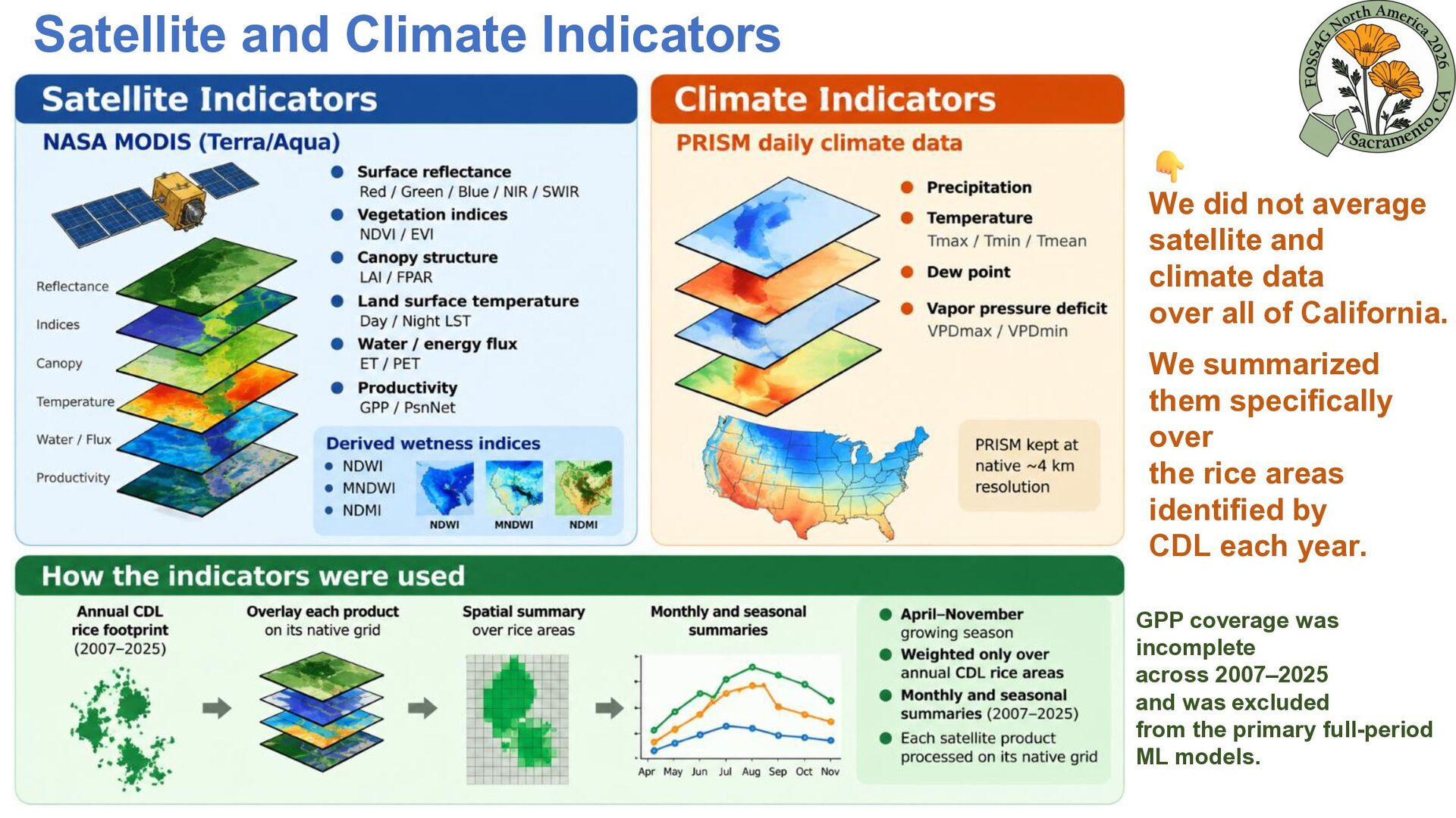
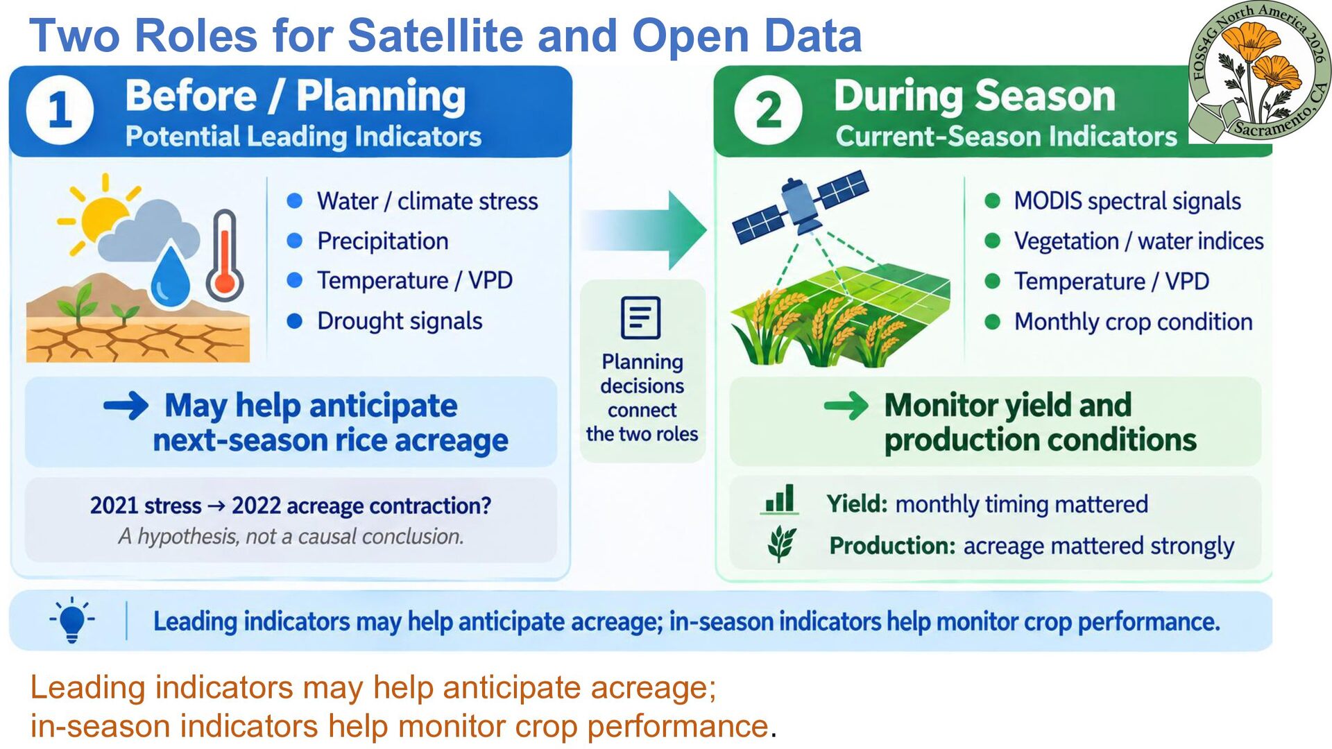
8. Satellite and Climate Indicators We did not average satellite and climate data over all of California. We summarized them specifically over the rice areas identified by CDL each year. GPP coverage was incomplete across 2007–2025 and was excluded from the primary full-period ML models.
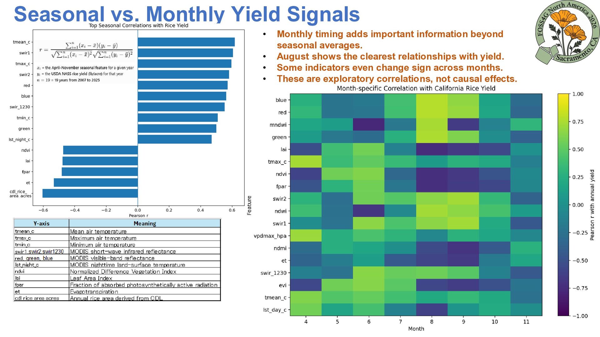
9. Seasonal vs. Monthly Yield Signals • • • • Monthly timing adds important information beyond seasonal averages. August shows the clearest relationships with yield. Some indicators even change sign across months. These are exploratory correlations, not causal effects.
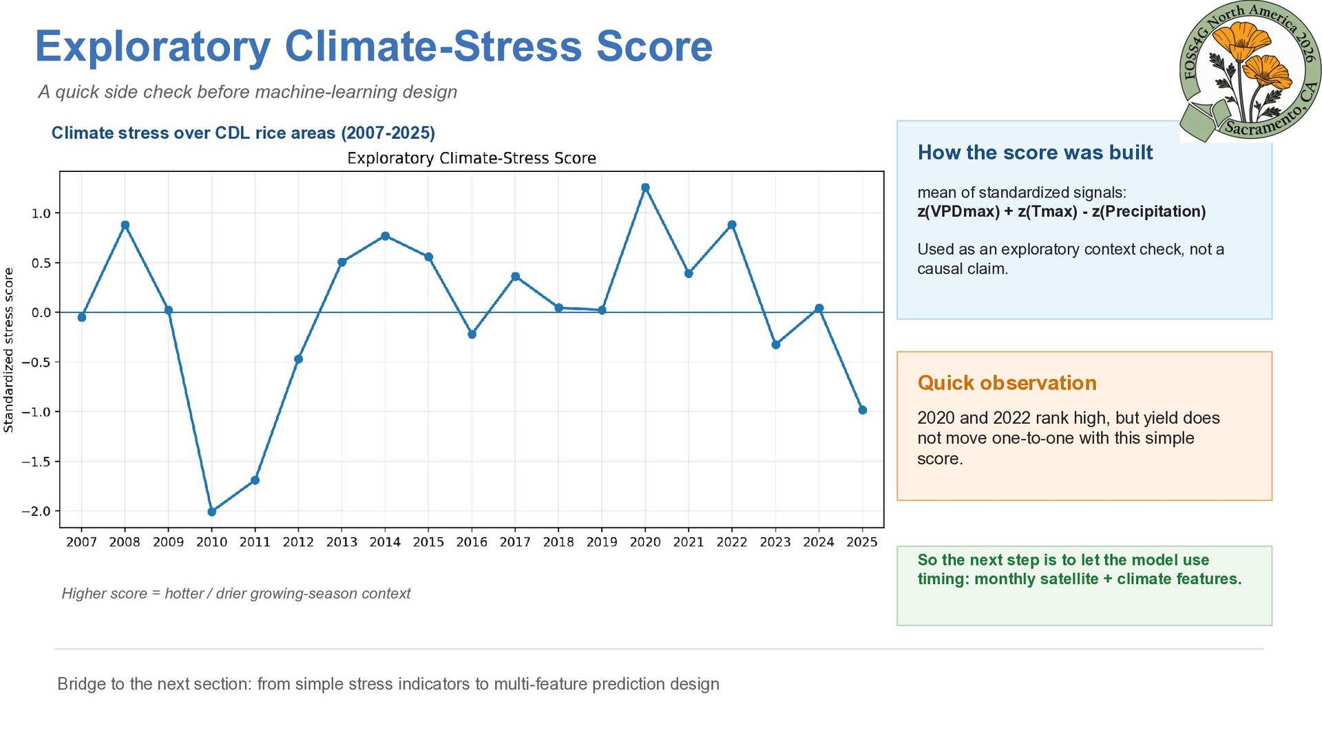
10. Exploratory Climate-Stress Score A quick side check before machine-learning design Climate stress over CDL rice areas (2007-2025) How the score was built mean of standardized signals: z(VPDmax) + z(Tmax) - z(Precipitation) Used as an exploratory context check, not a causal claim. Quick observation 2020 and 2022 rank high, but yield does not move one-to-one with this simple score. Higher score = hotter / drier growing-season context Bridge to the next section: from simple stress indicators to multi-feature prediction design So the next step is to let the model use timing: monthly satellite + climate features.
11. Machine-Learning Design Small sample, many features validation design matters more than model complexity.
12. Yield Prediction Best exploratory model Monthly timing+Random Forest RMSE: 212 lb/acre R²: 0.30 *Monthly timing outperformed seasonal averages (All predictions are held-out-year predictions) Why monthly? August visible-band signals and June MNDWI were repeatedly selected. Keeping monthly timing improved yield prediction.
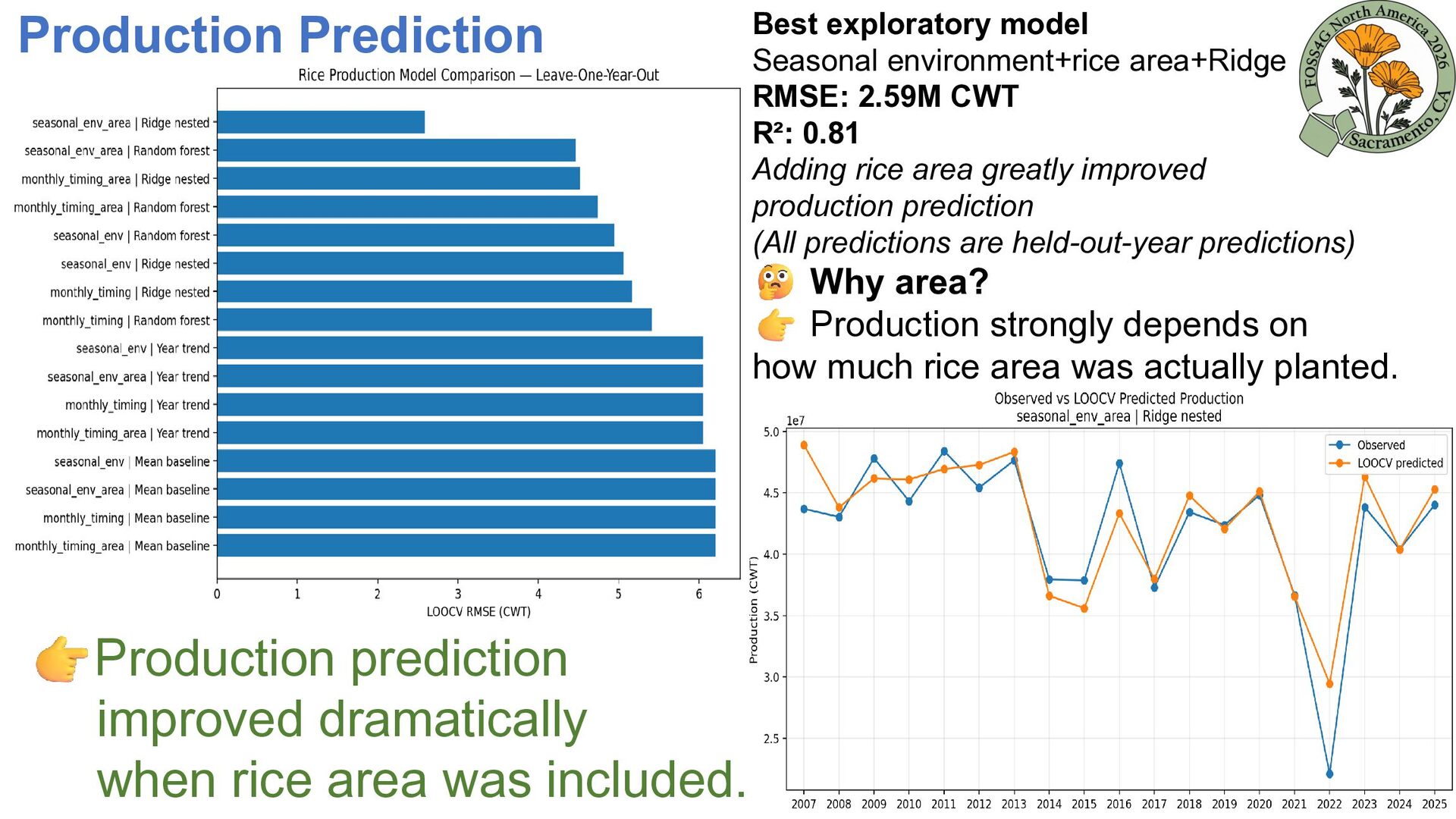
13. Production Prediction Best exploratory model Seasonal environment+rice area+Ridge RMSE: 2.59M CWT R²: 0.81 Adding rice area greatly improved production prediction (All predictions are held-out-year predictions) Why area? Production strongly depends on how much rice area was actually planted. Production prediction improved dramatically when rice area was included.
14. Two Roles for Satellite and Open Data Leading indicators may help anticipate acreage; in-season indicators help monitor crop performance.
15. Takeaways and Next Steps ★Slides & code are publicly available GitHub: https://github.com/takeofuture/foss4g_na_2026 Slides: ... More signals: precipitation · Tmax / Tmin · VPD · drought · soil moisture · reservoir levels · pests / diseases · crop phenology · lagged / time-series effects
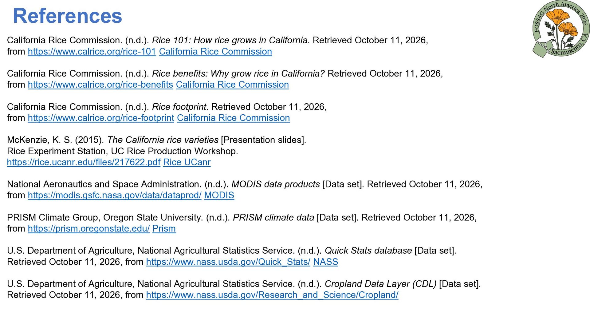
16. References California Rice Commission. (n.d.). Rice 101: How rice grows in California. Retrieved October 11, 2026, from https://www.calrice.org/rice-101 California Rice Commission California Rice Commission. (n.d.). Rice benefits: Why grow rice in California? Retrieved October 11, 2026, from https://www.calrice.org/rice-benefits California Rice Commission California Rice Commission. (n.d.). Rice footprint. Retrieved October 11, 2026, from https://www.calrice.org/rice-footprint California Rice Commission McKenzie, K. S. (2015). The California rice varieties [Presentation slides]. Rice Experiment Station, UC Rice Production Workshop. https://rice.ucanr.edu/files/217622.pdf Rice UCanr National Aeronautics and Space Administration. (n.d.). MODIS data products [Data set]. Retrieved October 11, 2026, from https://modis.gsfc.nasa.gov/data/dataprod/ MODIS PRISM Climate Group, Oregon State University. (n.d.). PRISM climate data [Data set]. Retrieved October 11, 2026, from https://prism.oregonstate.edu/ Prism U.S. Department of Agriculture, National Agricultural Statistics Service. (n.d.). Quick Stats database [Data set]. Retrieved October 11, 2026, from https://www.nass.usda.gov/Quick_Stats/ NASS U.S. Department of Agriculture, National Agricultural Statistics Service. (n.d.). Cropland Data Layer (CDL) [Data set]. Retrieved October 11, 2026, from https://www.nass.usda.gov/Research_and_Science/Cropland/
17. References Linquist, B., Al-Khatib, K., Brim-DeForest, W., Espe, M. B., Espino, L., Leinfelder-Miles, M., & Stogsdill, J. R. (2025). Predictors of high rice yields in a high-yielding environment: Lessons from a yield contest. Field Crops Research, 322, 109693. https://doi.org/10.1016/j.fcr.2024.109693 ScienceDirect Sharifi, H., Hijmans, R. J., Hill, J. E., & Linquist, B. A. (2017). Using stage-dependent temperature parameters to improve phenological model prediction accuracy in rice models. Crop Science, 57(1), 444–453. https://linquist.ucdavis.edu/sites/g/files/dgvnsk6581/files/inline-files/2016-Sharifi-et-al-Crop-Science.pdf
18. Appendix 1 – Workflow and Programs GitHub: https://github.com/takeofuture/foss4g_na_2026
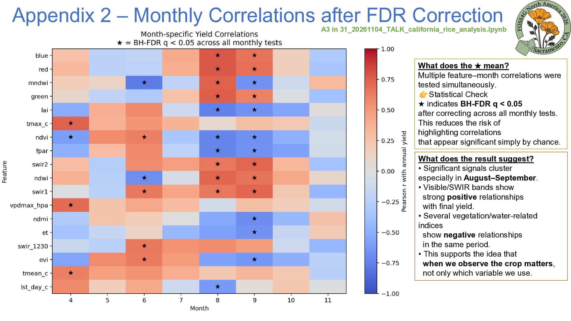
19. Appendix 2 – Monthly Correlations after FDR Correction A3 in 31_20261104_TALK_california_rice_analysis.ipynb What does the ★ mean? Multiple feature–month correlations were tested simultaneously. Statistical Check ★ indicates BH-FDR q < 0.05 after correcting across all monthly tests. This reduces the risk of highlighting correlations that appear significant simply by chance. What does the result suggest? • Significant signals cluster especially in August–September. • Visible/SWIR bands show strong positive relationships with final yield. • Several vegetation/water-related indices show negative relationships in the same period. • This supports the idea that when we observe the crop matters, not only which variable we use.
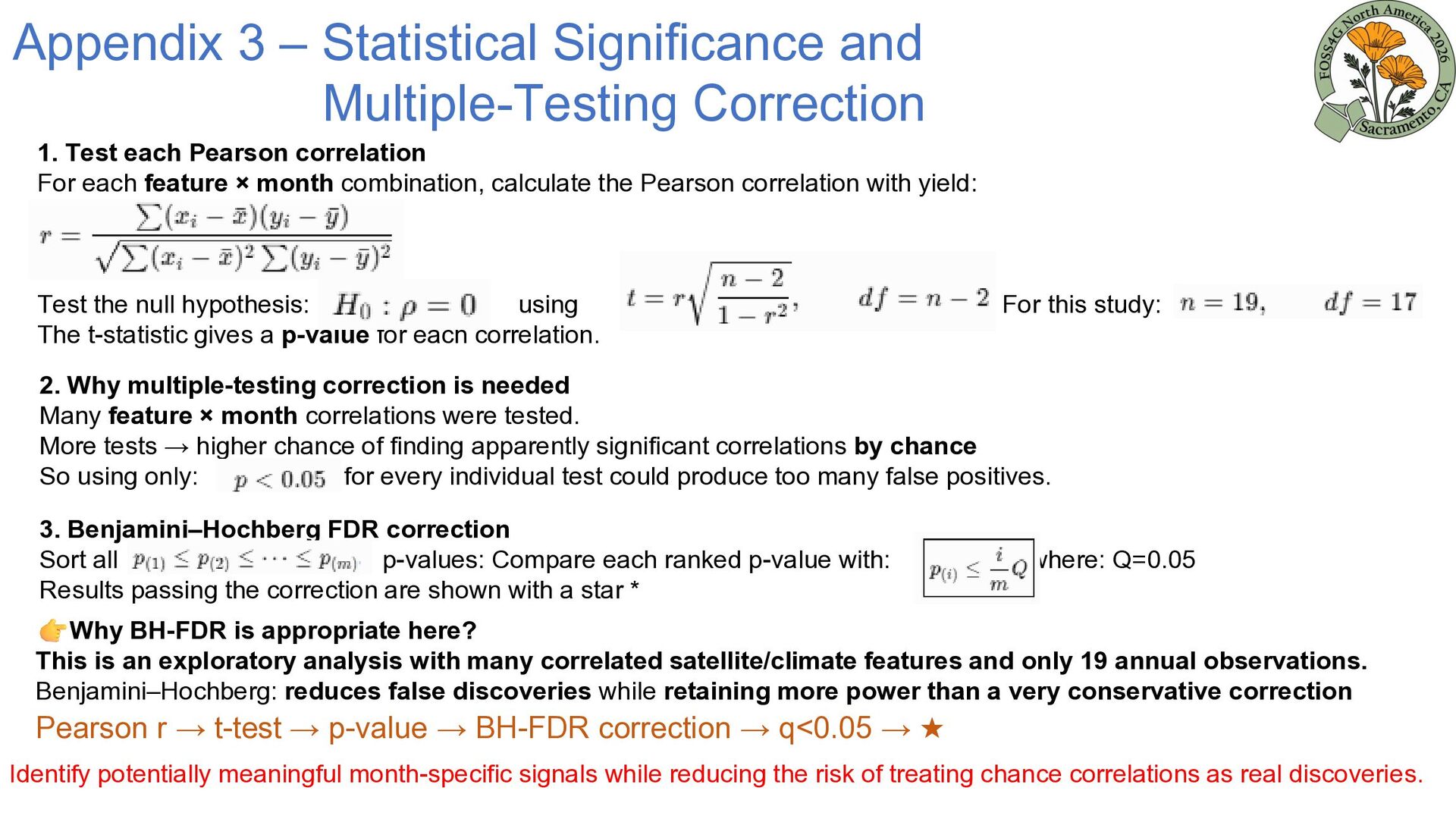
20. Appendix 3 – Statistical Significance and Multiple-Testing Correction 1. Test each Pearson correlation For each feature × month combination, calculate the Pearson correlation with yield: Test the null hypothesis: using The t-statistic gives a p-value for each correlation. For this study: 2. Why multiple-testing correction is needed Many feature × month correlations were tested. More tests → higher chance of finding apparently significant correlations by chance So using only: for every individual test could produce too many false positives. 3. Benjamini–Hochberg FDR correction Sort all p-values: Compare each ranked p-value with: Results passing the correction are shown with a star * where: Q=0.05 Why BH-FDR is appropriate here? This is an exploratory analysis with many correlated satellite/climate features and only 19 annual observations. Benjamini–Hochberg: reduces false discoveries while retaining more power than a very conservative correction Pearson r → t-test → p-value → BH-FDR correction → q<0.05 → ★ Identify potentially meaningful month-specific signals while reducing the risk of treating chance correlations as real discoveries.
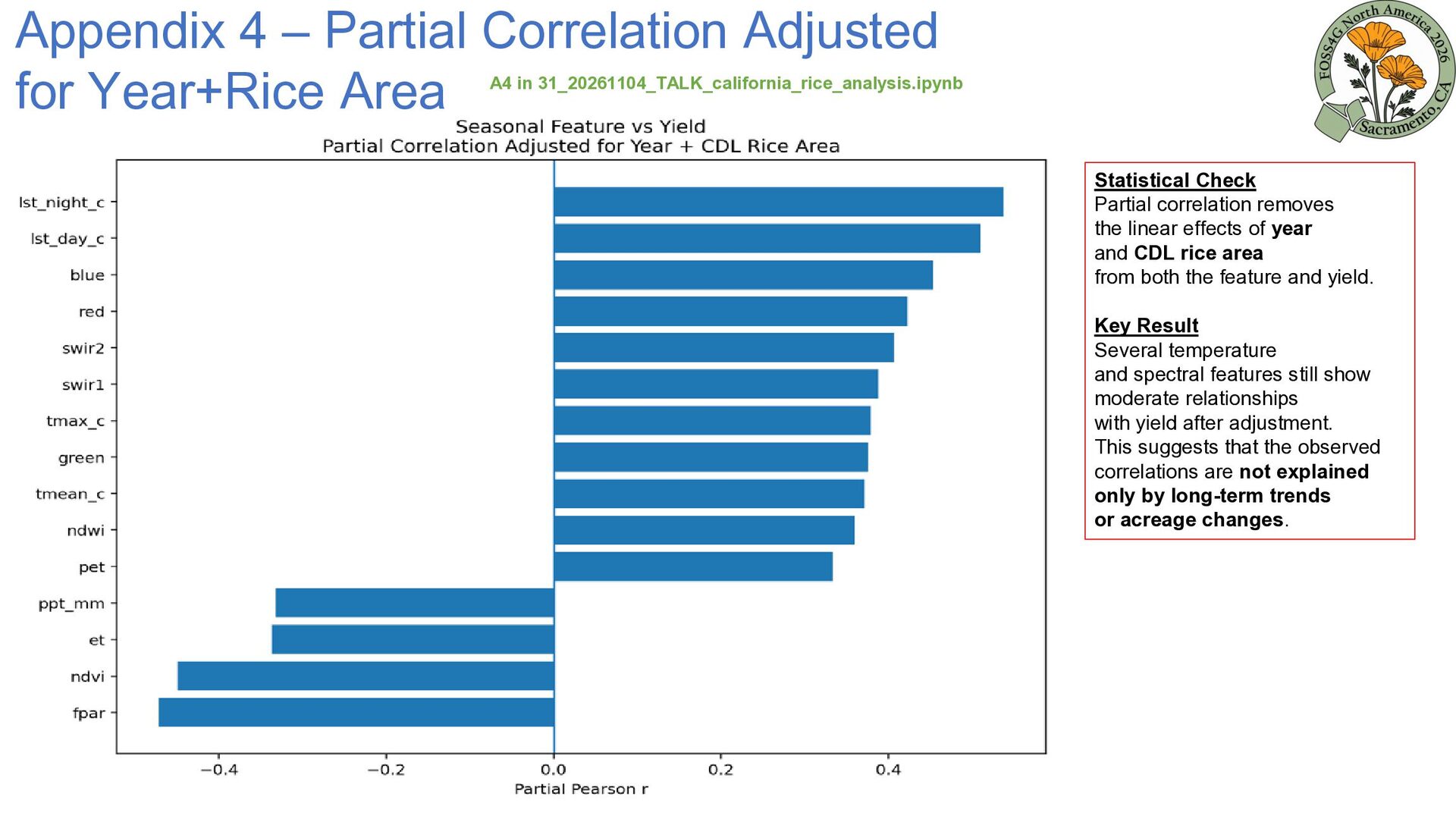
21. Appendix 4 – Partial Correlation Adjusted for Year+Rice Area A4 in 31_20261104_TALK_california_rice_analysis.ipynb Statistical Check Partial correlation removes the linear effects of year and CDL rice area from both the feature and yield. Key Result Several temperature and spectral features still show moderate relationships with yield after adjustment. This suggests that the observed correlations are not explained only by long-term trends or acreage changes.
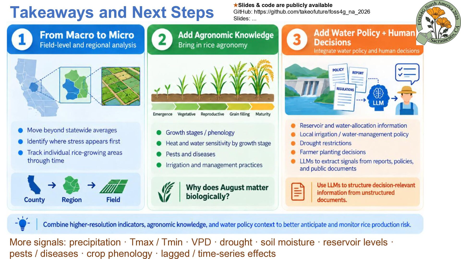
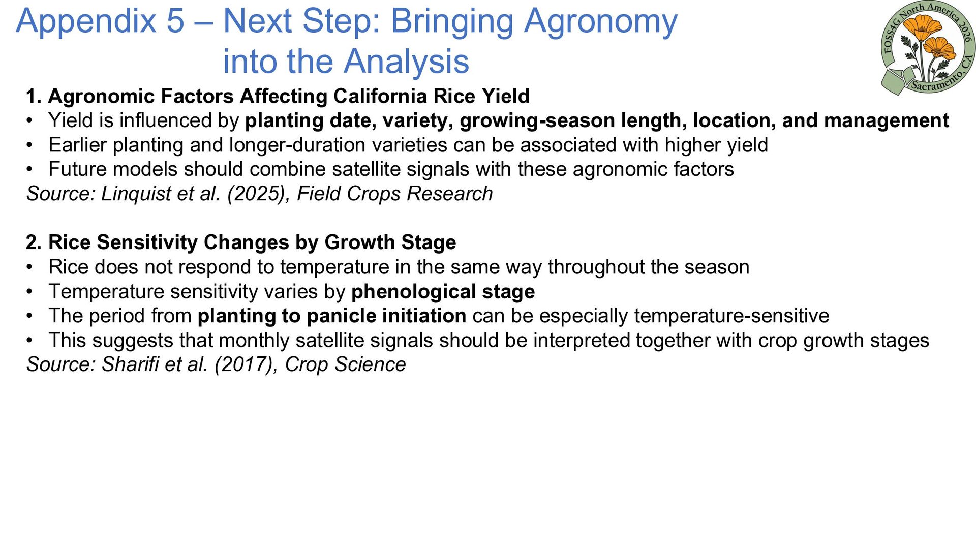
22. Appendix 5 – Next Step: Bringing Agronomy into the Analysis 1. Agronomic Factors Affecting California Rice Yield • Yield is influenced by planting date, variety, growing-season length, location, and management • Earlier planting and longer-duration varieties can be associated with higher yield • Future models should combine satellite signals with these agronomic factors Source: Linquist et al. (2025), Field Crops Research 2. Rice Sensitivity Changes by Growth Stage • Rice does not respond to temperature in the same way throughout the season • Temperature sensitivity varies by phenological stage • The period from planting to panicle initiation can be especially temperature-sensitive • This suggests that monthly satellite signals should be interpreted together with crop growth stages Source: Sharifi et al. (2017), Crop Science
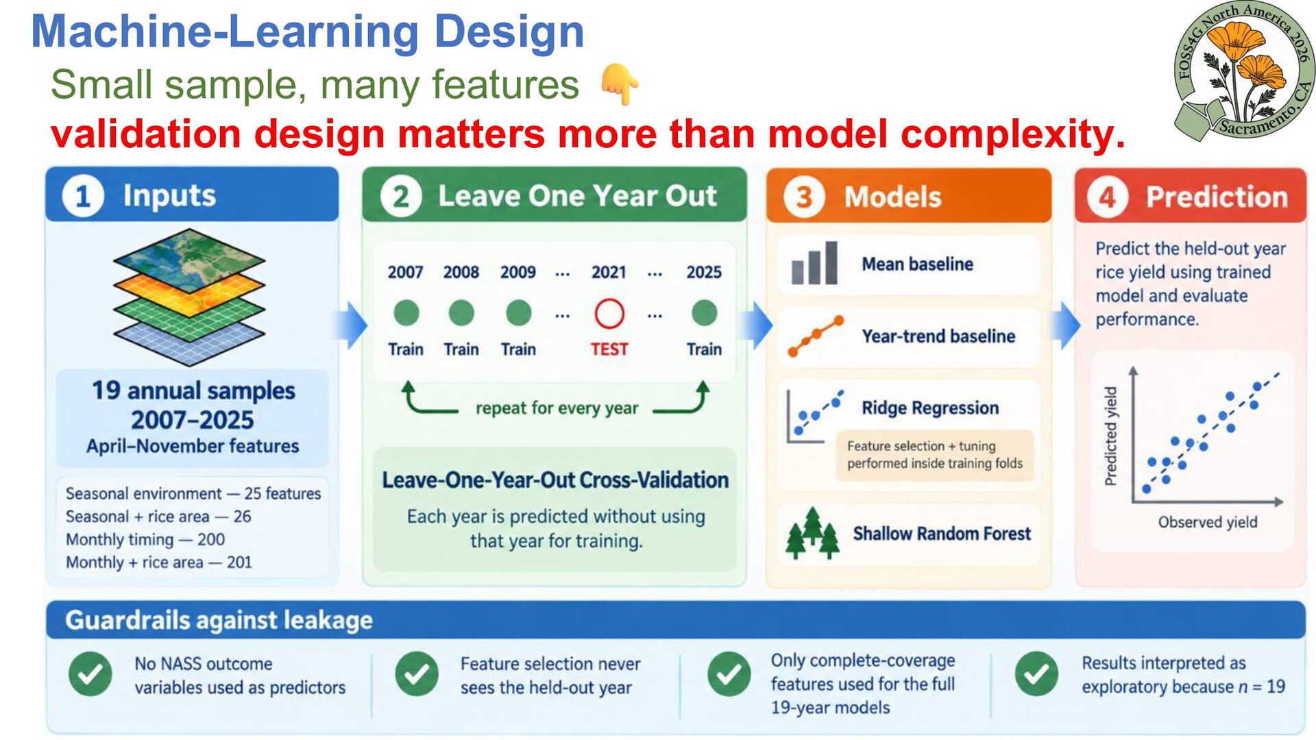
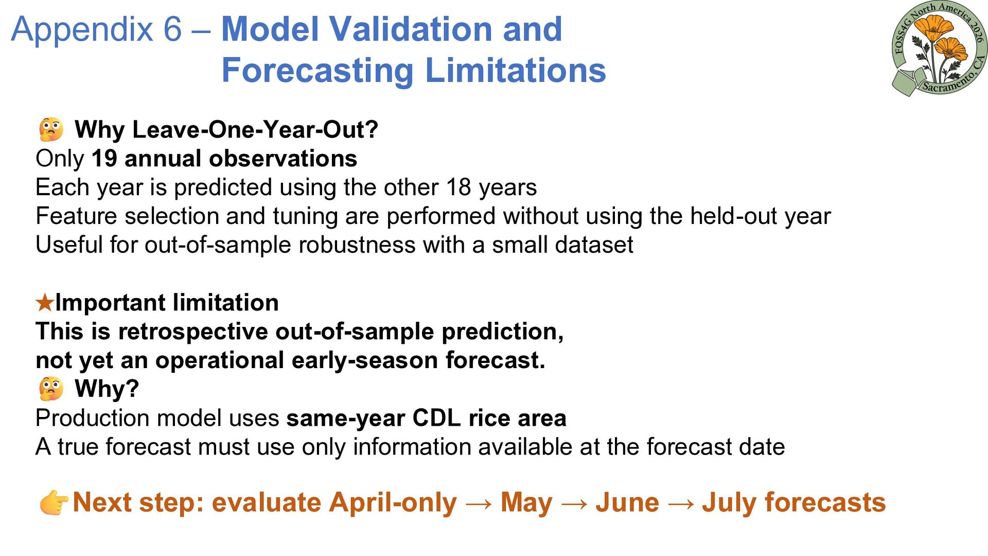
23. Appendix 6 – Model Validation and Forecasting Limitations Why Leave-One-Year-Out? Only 19 annual observations Each year is predicted using the other 18 years Feature selection and tuning are performed without using the held-out year Useful for out-of-sample robustness with a small dataset ★Important limitation This is retrospective out-of-sample prediction, not yet an operational early-season forecast. Why? Production model uses same-year CDL rice area A true forecast must use only information available at the forecast date Next step: evaluate April-only → May → June → July forecasts
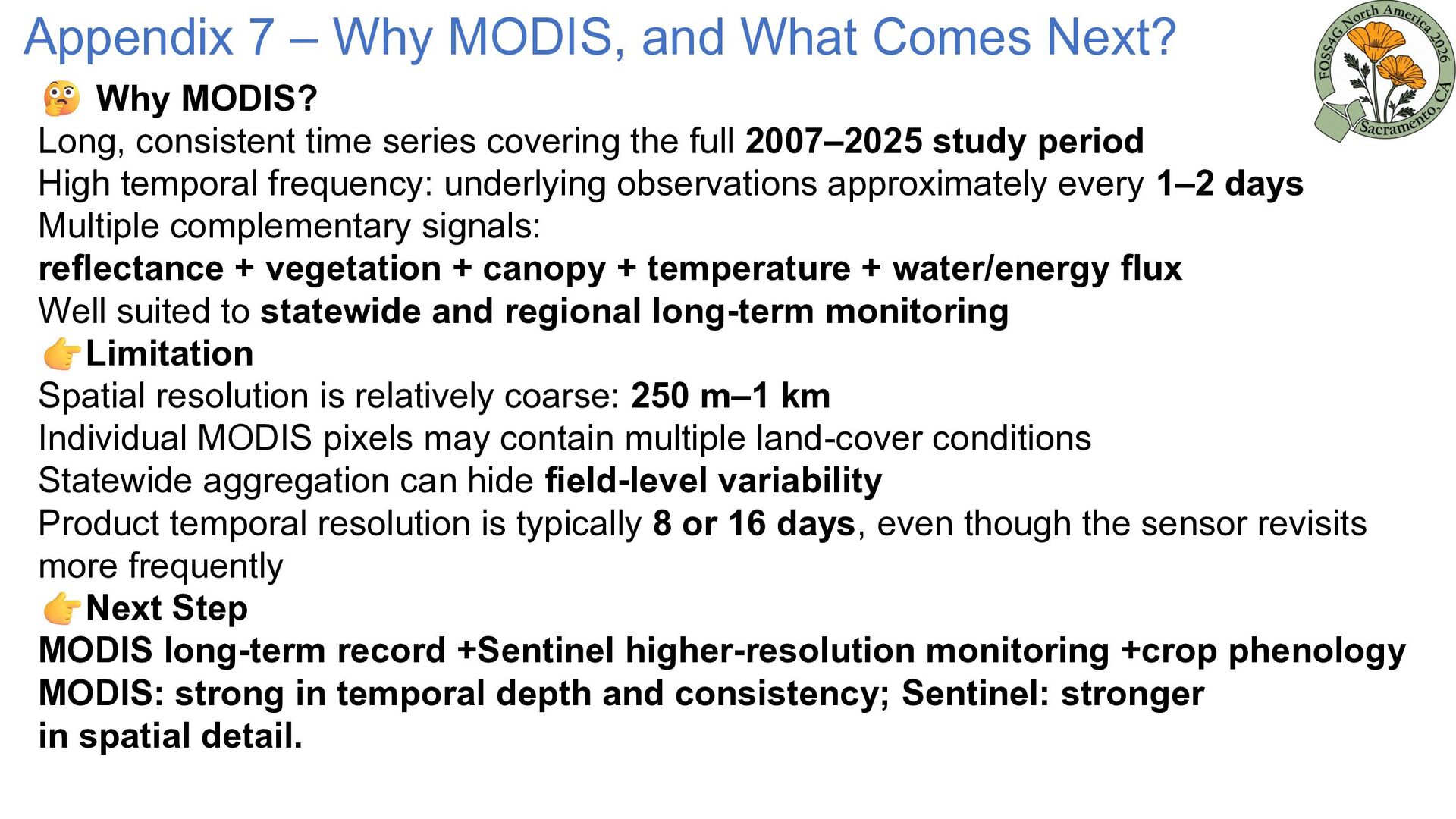
24. Appendix 7 – Why MODIS, and What Comes Next? Why MODIS? Long, consistent time series covering the full 2007–2025 study period High temporal frequency: underlying observations approximately every 1–2 days Multiple complementary signals: reflectance + vegetation + canopy + temperature + water/energy flux Well suited to statewide and regional long-term monitoring Limitation Spatial resolution is relatively coarse: 250 m–1 km Individual MODIS pixels may contain multiple land-cover conditions Statewide aggregation can hide field-level variability Product temporal resolution is typically 8 or 16 days, even though the sensor revisits more frequently Next Step MODIS long-term record +Sentinel higher-resolution monitoring +crop phenology MODIS: strong in temporal depth and consistency; Sentinel: stronger in spatial detail.