for Graphs, and Superconcentrators”. Journal of Combinatorial Theory, Series B 38.1, pp. 73–88. S. Arora, E. Hazan, S. Kale (2010). “O( √ log n)-Approximation to SPARSEST CUT in O(n2) Time”. SIAM Journal on Computing 39.5, pp. 1748–1771. S. Arora, S. Kale (2016). “A Combinatorial, Primal-Dual Approach to Semidefinite Programs”. Journal of the ACM 63.2, pp. 1–35. S. Arora, S. Rao, U. Vazirani (2009). “Expander Flows, Geometric Embeddings and Graph Partitioning”. Journal of the ACM 56.2, pp. 1–37. S. Kale (2007). “Efficient algorithms using the multiplicative weights update method”. PhD thesis. Princeton University. R. Khandekar, S. Rao, U. Vazirani (2009). “Graph Partitioning Using Single Commodity Flows”. Journal of the ACM 56.4, pp. 1–15. T. Leighton, S. Rao (1999). “Multicommodity Max-Flow Min-Cut Theorems and Their Use in Designing Approximation Algorithms”. Journal of the ACM 46.6, pp. 787–832. L. Orecchia, L. J. Schulman, U. V. Vazirani, N. K. Vishnoi (2008). “On partitioning graphs via single commodity flows”. In: Proceedings of the fortieth annual ACM symposium on Theory of computing, pp. 461–470. L. Trevisan (2012). “Max Cut and the Smallest Eigenvalue”. SIAM Journal on Computing 41.6, pp. 1769–1786. 1 / 1
![Cheeger inequality Cheeger inequality for λ2 [Alon, Milman 1985] λ2](https://files.speakerdeck.com/presentations/98a17cdd9d8b453e9786f30450c7bd0e/slide_3.jpg)
![Cheeger inequality Cheeger inequality for λ2 [Alon, Milman 1985] λ2](https://files.speakerdeck.com/presentations/98a17cdd9d8b453e9786f30450c7bd0e/slide_4.jpg)
![Cheeger inequality Cheeger inequality for λn [Trevisan 2012] 2 −](https://files.speakerdeck.com/presentations/98a17cdd9d8b453e9786f30450c7bd0e/slide_5.jpg)
![Cheeger inequality Cheeger inequality for λn [Trevisan 2012] 2 −](https://files.speakerdeck.com/presentations/98a17cdd9d8b453e9786f30450c7bd0e/slide_6.jpg)
![Cheeger inequality Cheeger inequality for λn [Trevisan 2012] 2 −](https://files.speakerdeck.com/presentations/98a17cdd9d8b453e9786f30450c7bd0e/slide_7.jpg)
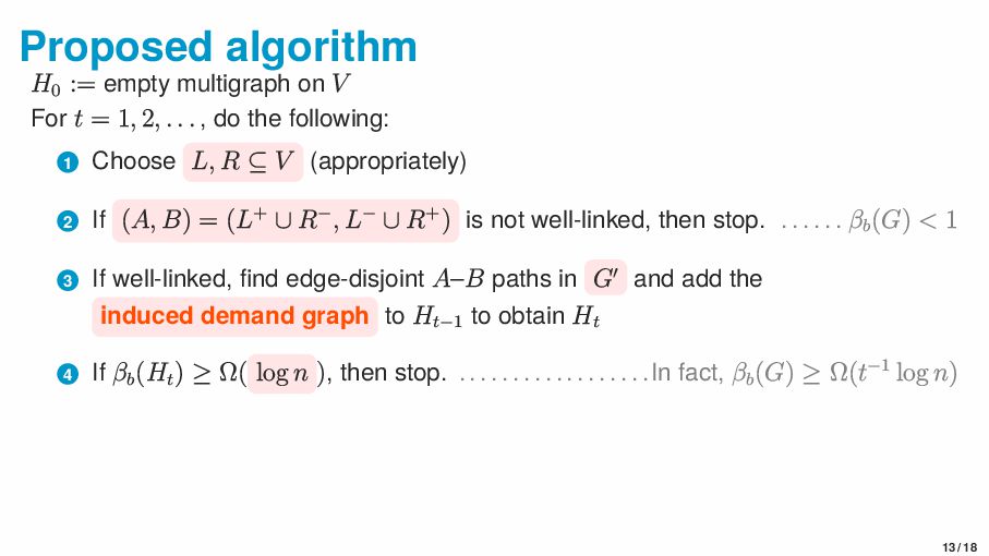
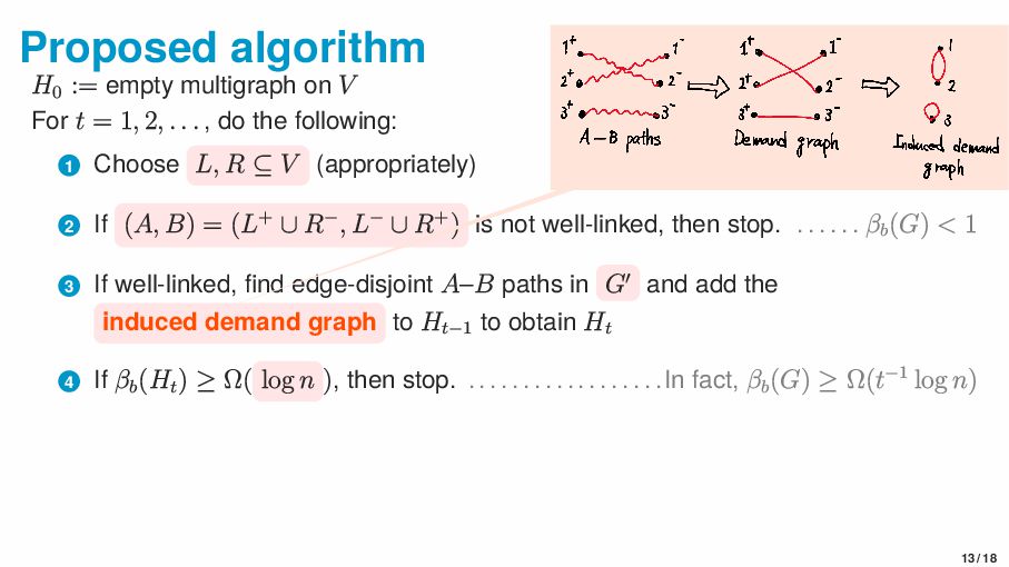
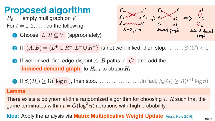
![Cut-matching game [Khandekar, Rao, U. Vazirani 2009] H0 := empty](https://files.speakerdeck.com/presentations/98a17cdd9d8b453e9786f30450c7bd0e/slide_18.jpg)
![Cut-matching game [Khandekar, Rao, U. Vazirani 2009] H0 := empty](https://files.speakerdeck.com/presentations/98a17cdd9d8b453e9786f30450c7bd0e/slide_19.jpg)
![Cut-matching game [Khandekar, Rao, U. Vazirani 2009] H0 := empty](https://files.speakerdeck.com/presentations/98a17cdd9d8b453e9786f30450c7bd0e/slide_20.jpg)