• Developers should attempt to minimize the negative effects on water quality. • In order to do this, site specific relationships of the water quality and development patterns need to be understood by planners and developers. Site specific studies to assess water quality and development relationship
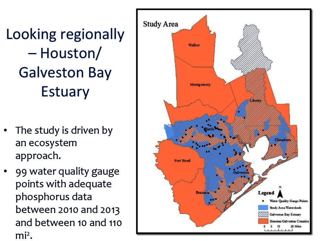
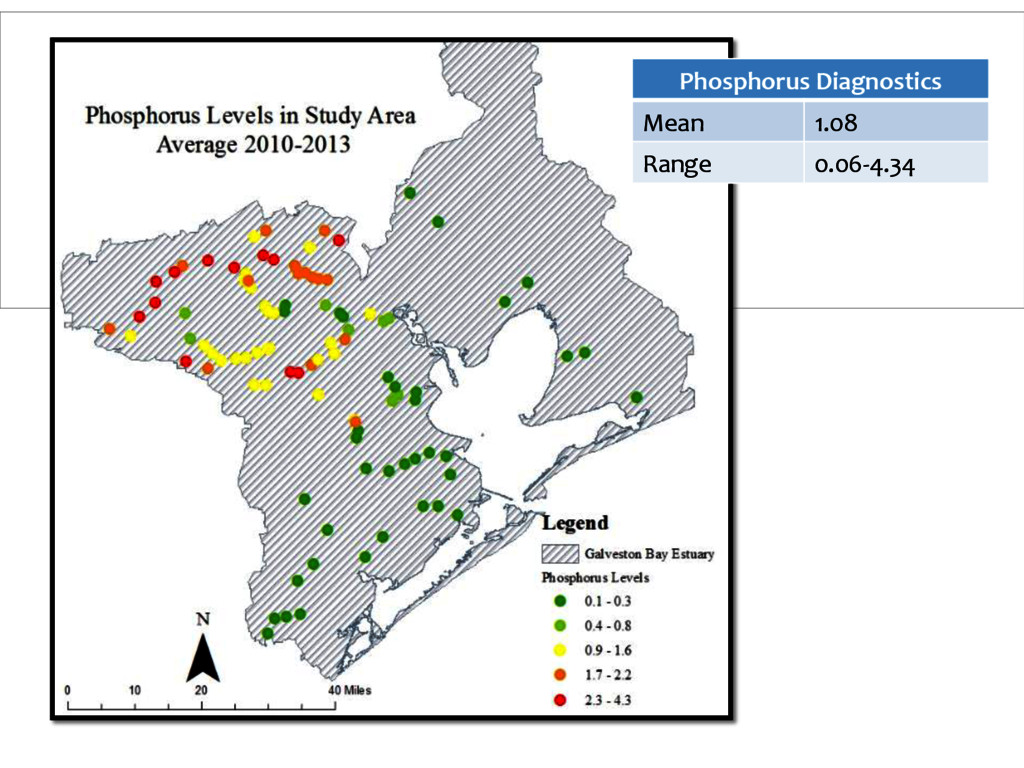
• The study is driven by an ecosystem approach. • 99 water quality gauge points with adequate phosphorus data between 2010 and 2013 and between 10 and 110 mi2.
in the U.S. • About 6.5 million people and growing in the Houston/ Galveston region (Houston-‐Galveston Area Council, 2014) • The largest growth of any metro center in the United States between 2000 and 2010 (US Census Bureau, 2012) Fast growing population accelerates anthropogenic effects
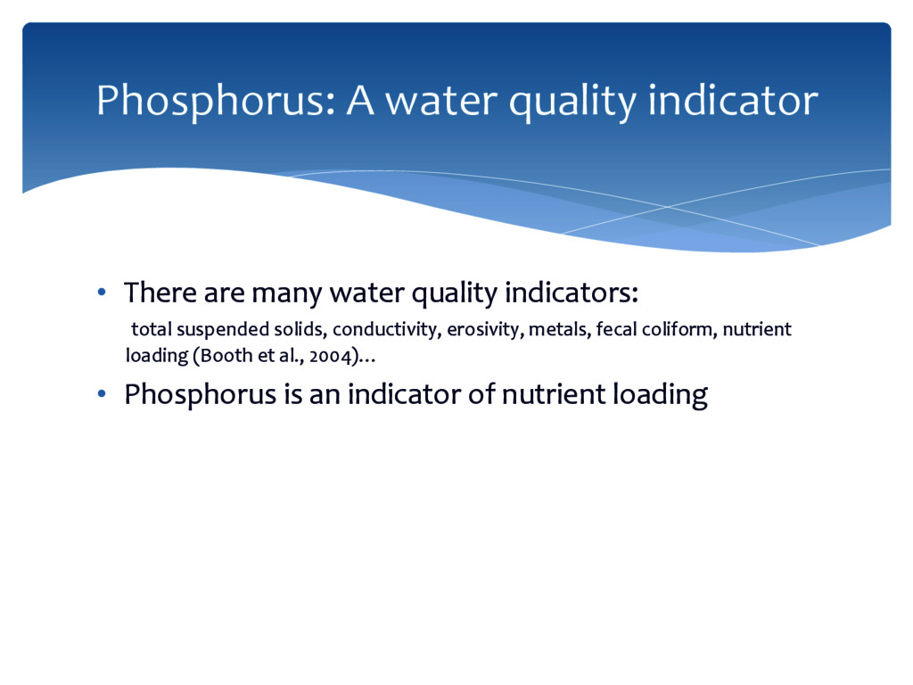
solids, conductivity, erosivity, metals, fecal coliform, nutrient loading (Booth et al., 2004)… • Phosphorus is an indicator of nutrient loading Phosphorus: A water quality indicator
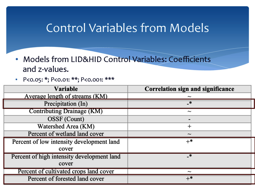
be used as control variables in the statistical models • Account for seasonal variability • Averages will be used to remove these variations. Other factors influencing water quality
2004; Halstead et al., 2014) • Look at the impact of development on specific water quality variables such as nitrogen, phosphorus, and sediment (Coulter et al., 2004; Zampella et al., 2007). • Impervious surface and how the nutrient loading is affected when impervious surface area increases (Dietz and Clausen, 2008). Previous Research on the relationship between water quality and development
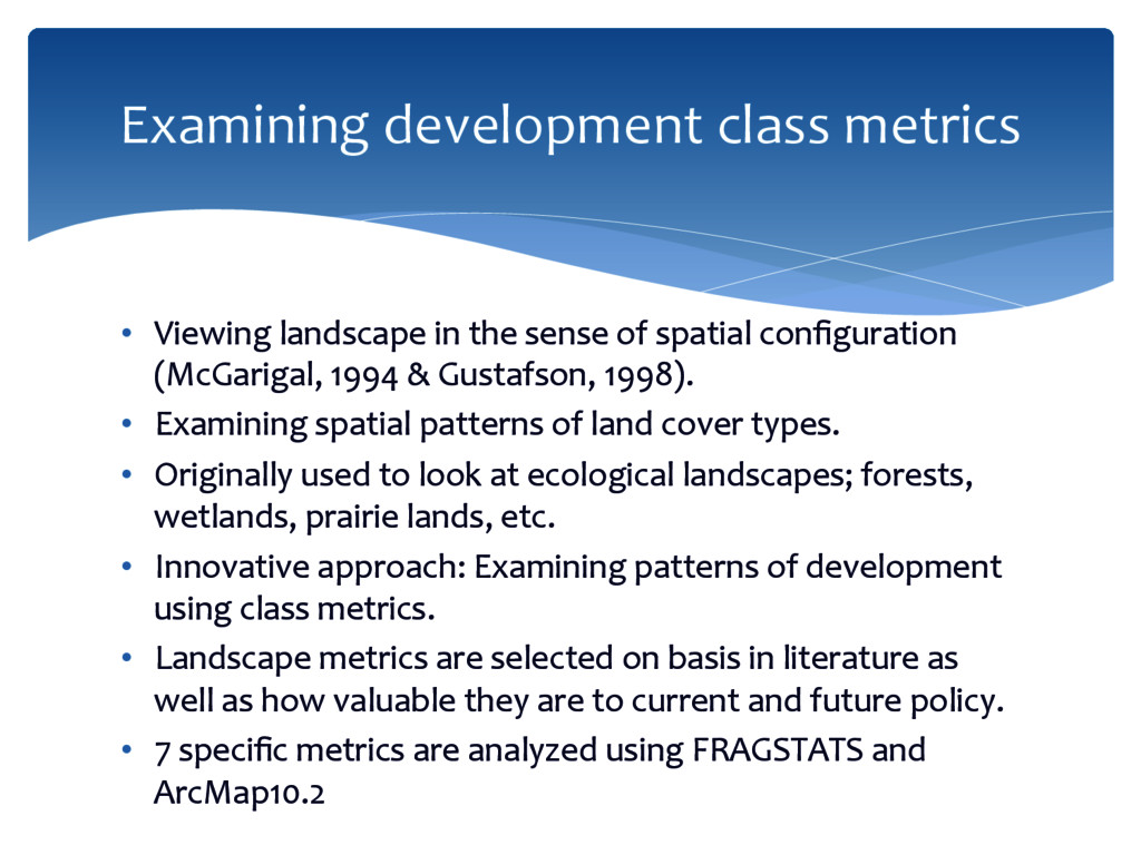
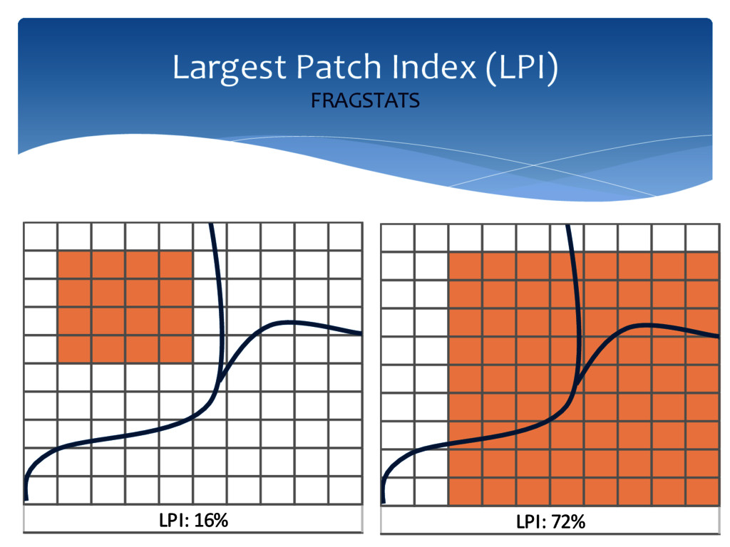
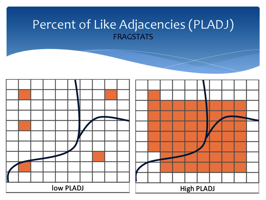
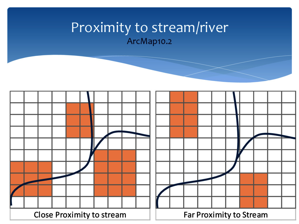
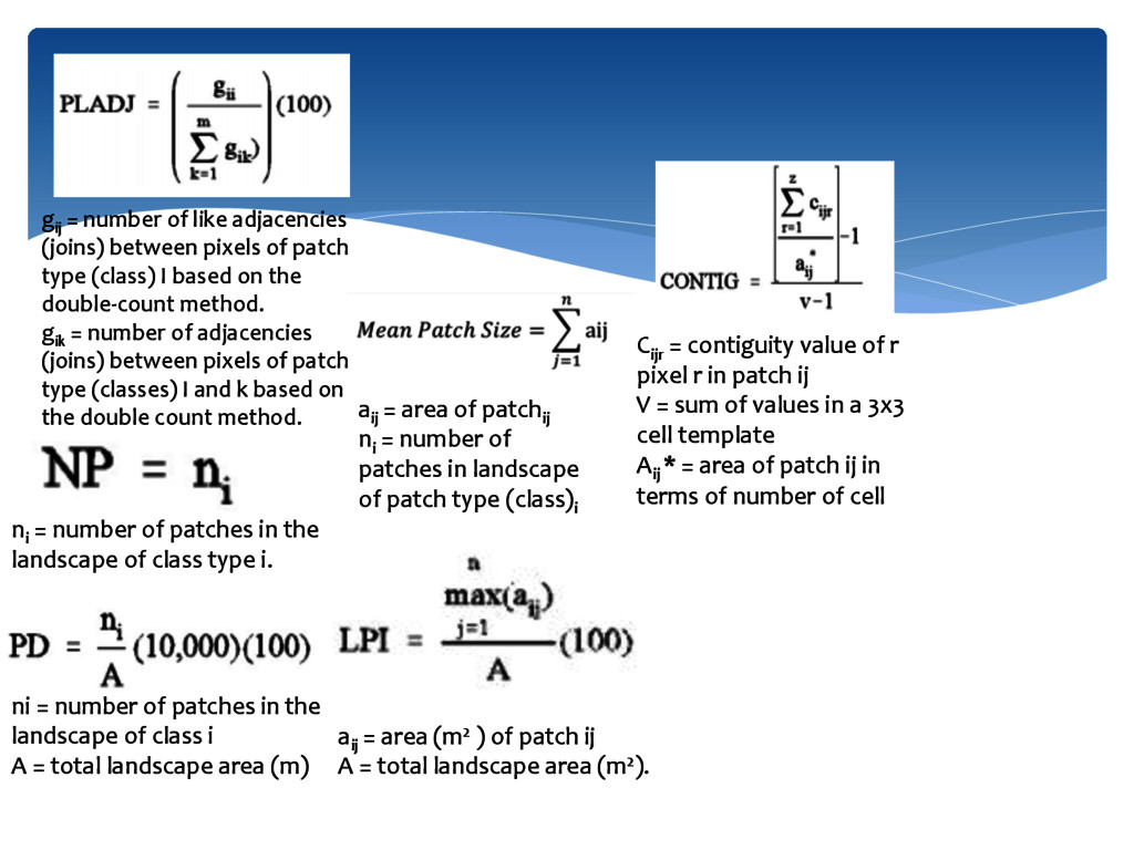
(McGarigal, 1994 & Gustafson, 1998). • Examining spatial patterns of land cover types. • Originally used to look at ecological landscapes; forests, wetlands, prairie lands, etc. • Innovative approach: Examining patterns of development using class metrics. • Landscape metrics are selected on basis in literature as well as how valuable they are to current and future policy. • 7 specific metrics are analyzed using FRAGSTATS and ArcMap10.2 Examining development class metrics
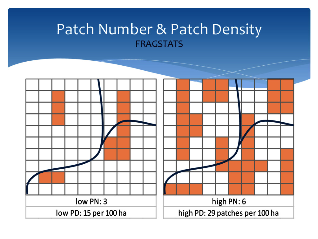
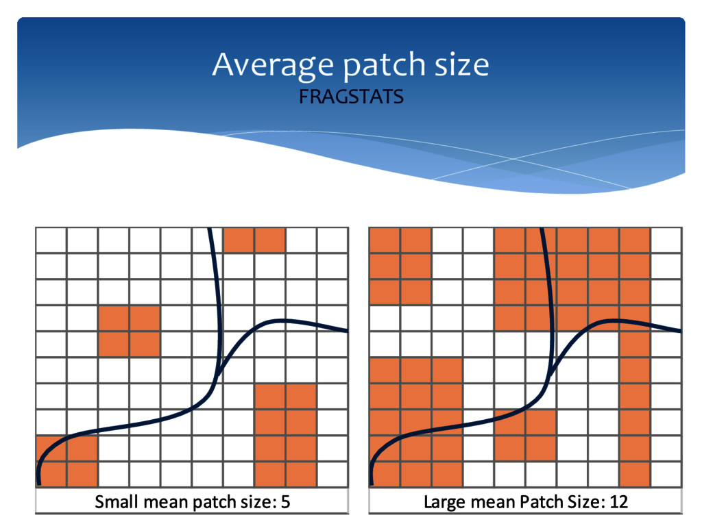
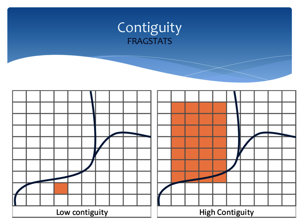
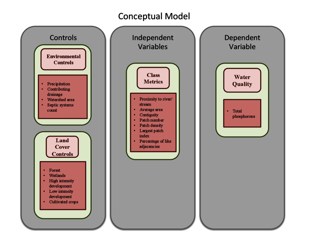
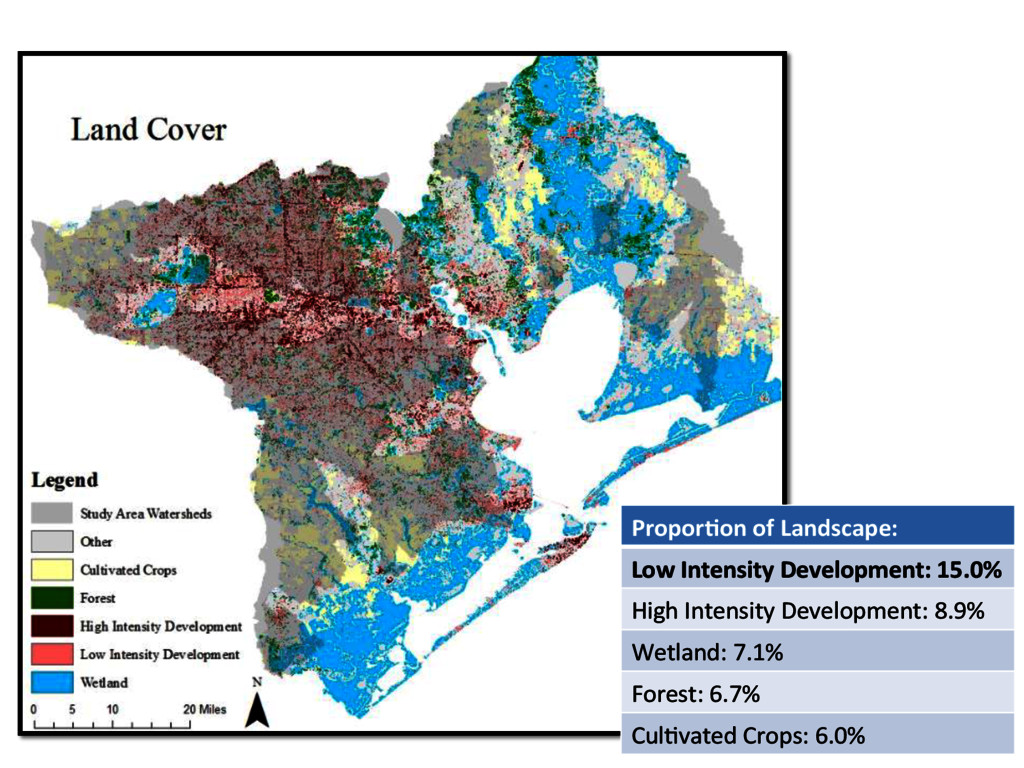
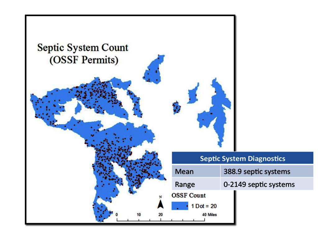
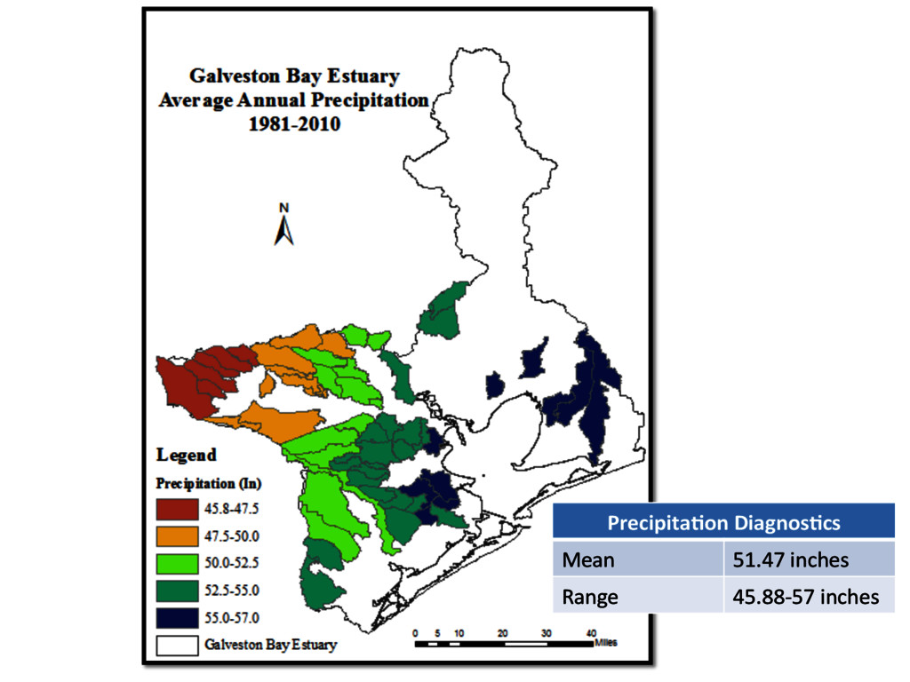
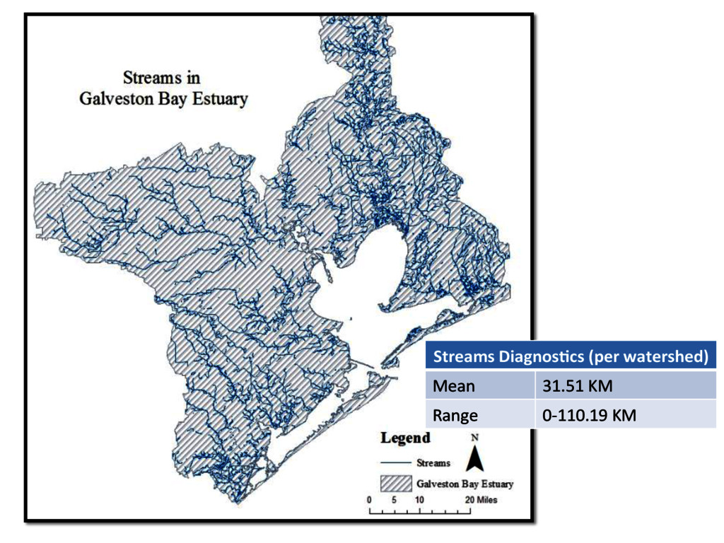
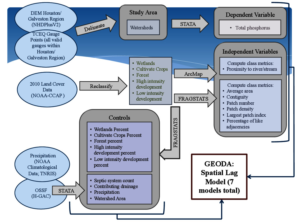
Conceptual Model • Forest • Wetlands • High intensity development • Low intensity development • Cultivated crops Land Cover Controls • Total phosphorous Water Quality • Proximity to river/ stream • Average area • Contiguity • Patch number • Patch density • Largest patch index • Percentage of like adjacencies Class Metrics • Precipitation • Contributing drainage • Watershed area • Septic systems count Environmental Controls
) DEM Houston/ Galveston Region (NHDPlusV2) TCEQ Gauge Points (all valid gauges within Houston/ Galveston Region) Reclassify • Wetlands • Cultivate Crops • Forest • High intensity development • Low intensity development Delineate GEODA: Spatial Lag Model (7 models total) Independent Variables Compute class metrics: • Average area • Contiguity • Patch number • Patch density • Largest patch index • Percentage of like adjacencies Compute class metrics: • Proximity to river/stream STATA Dependent Variable • Total phosphorus Precipitation (NOAA Climatological Data; TNRIS) Controls • Wetlands Percent • Cultivate Crops Percent • Forest percent • High intensity development percent • Low intensity development percent • Septic system count • Contributing drainage • Precipitation • Watershed Area ArcMap FRAGSTATS STATA Watersheds
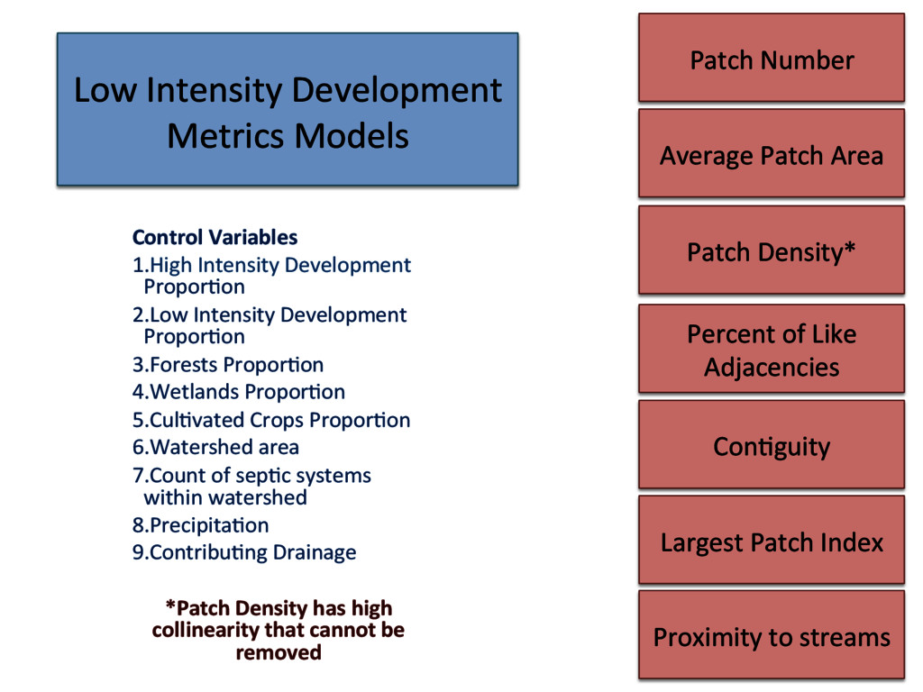
to streams Patch Number Average Patch Area Percent of Like Adjacencies Low Intensity Development Metrics Models Control Variables 1. High Intensity Development ProporLon 2. Low Intensity Development ProporLon 3. Forests ProporLon 4. Wetlands ProporLon 5. CulLvated Crops ProporLon 6. Watershed area 7. Count of sepLc systems within watershed 8. PrecipitaLon 9. ContribuLng Drainage *Patch Density has high collinearity that cannot be removed
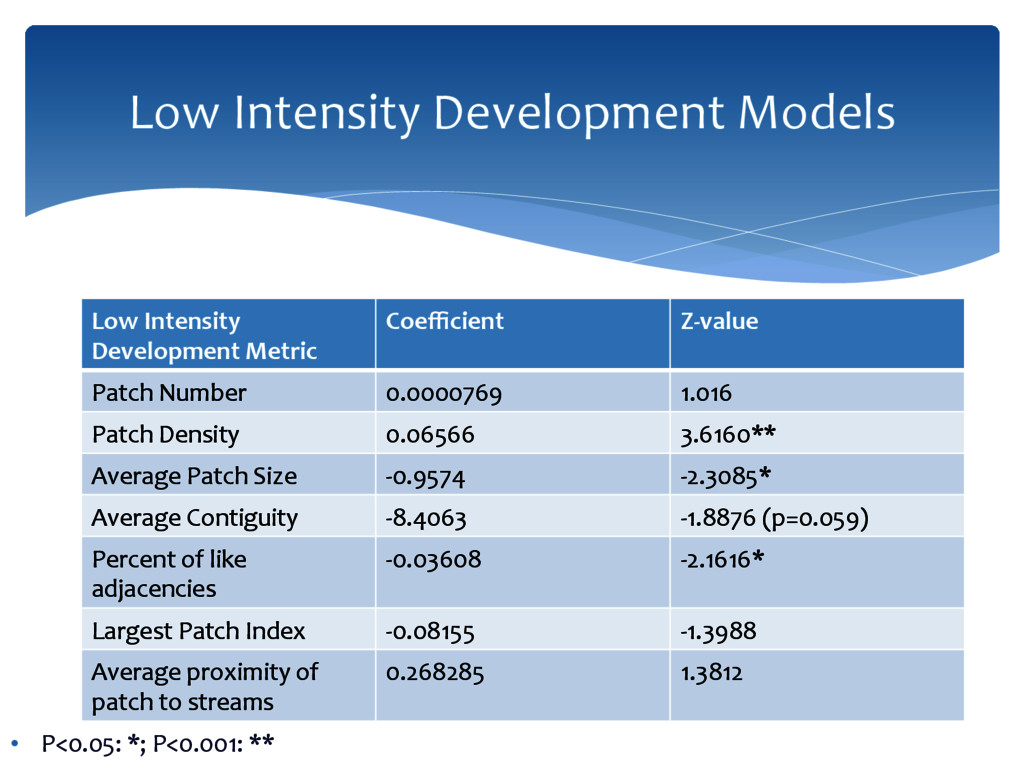
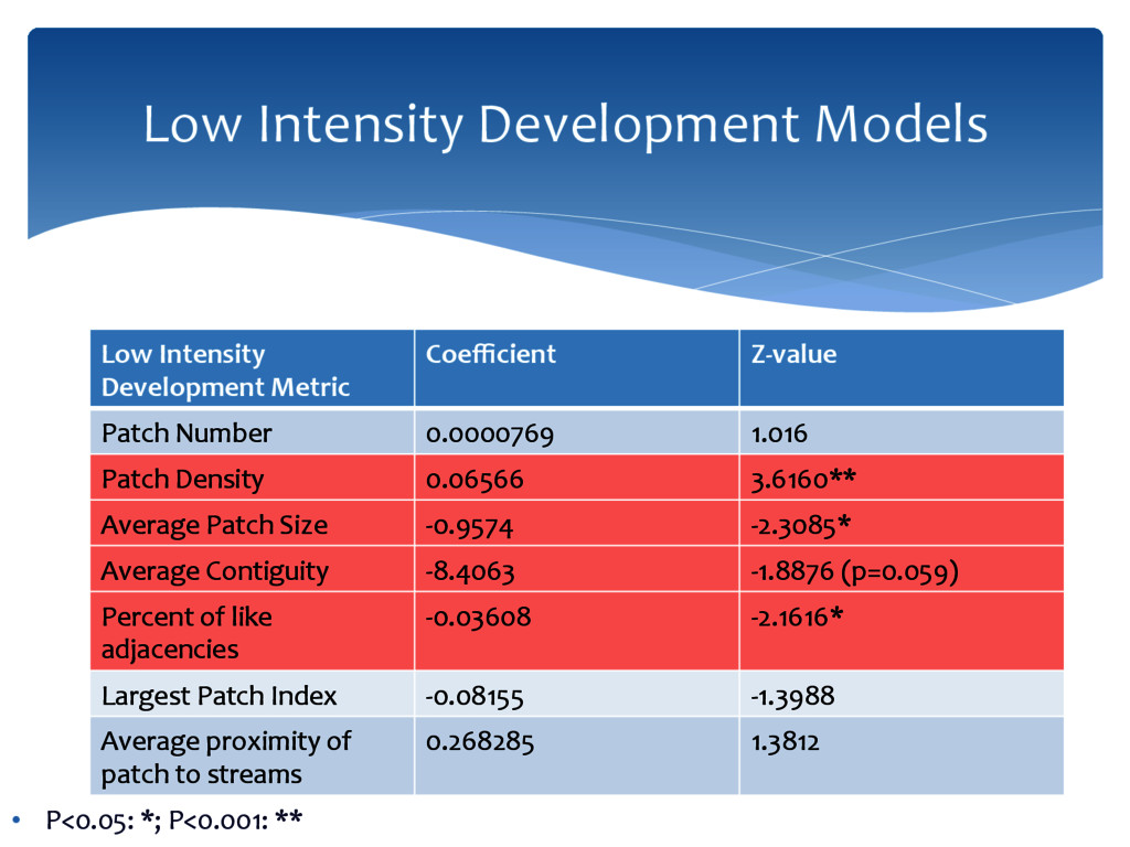
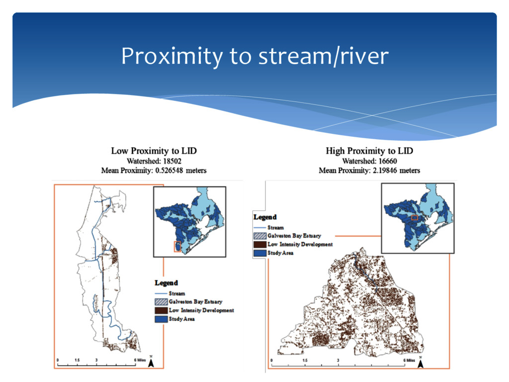
Low Intensity Development Metric Coefficient Z-‐value Patch Number 0.0000769 1.016 Patch Density 0.06566 3.6160** Average Patch Size -‐0.9574 -‐2.3085* Average Contiguity -‐8.4063 -‐1.8876 (p=0.059) Percent of like adjacencies -‐0.03608 -‐2.1616* Largest Patch Index -‐0.08155 -‐1.3988 Average proximity of patch to streams 0.268285 1.3812
Low Intensity Development Metric Coefficient Z-‐value Patch Number 0.0000769 1.016 Patch Density 0.06566 3.6160** Average Patch Size -‐0.9574 -‐2.3085* Average Contiguity -‐8.4063 -‐1.8876 (p=0.059) Percent of like adjacencies -‐0.03608 -‐2.1616* Largest Patch Index -‐0.08155 -‐1.3988 Average proximity of patch to streams 0.268285 1.3812
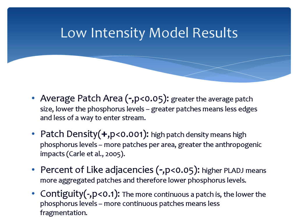
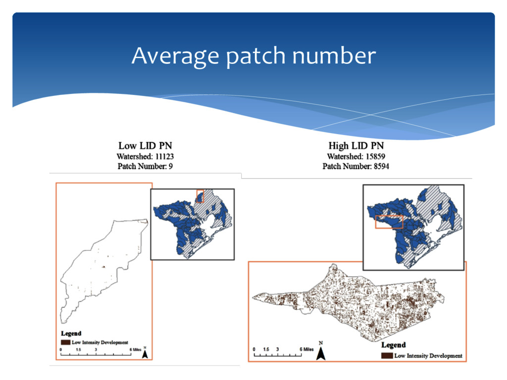
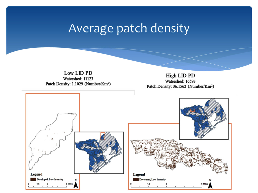
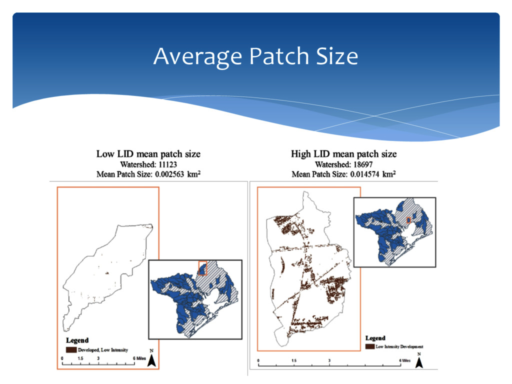
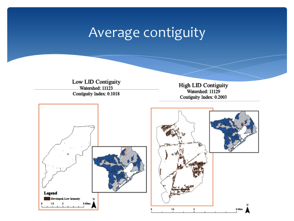
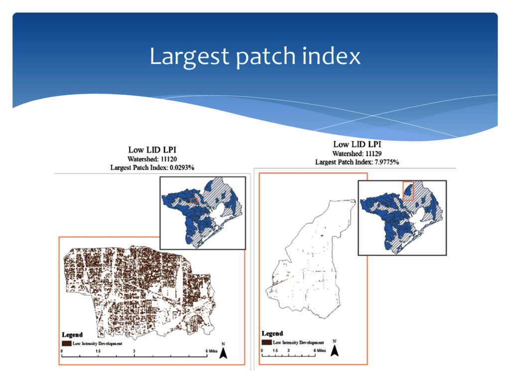
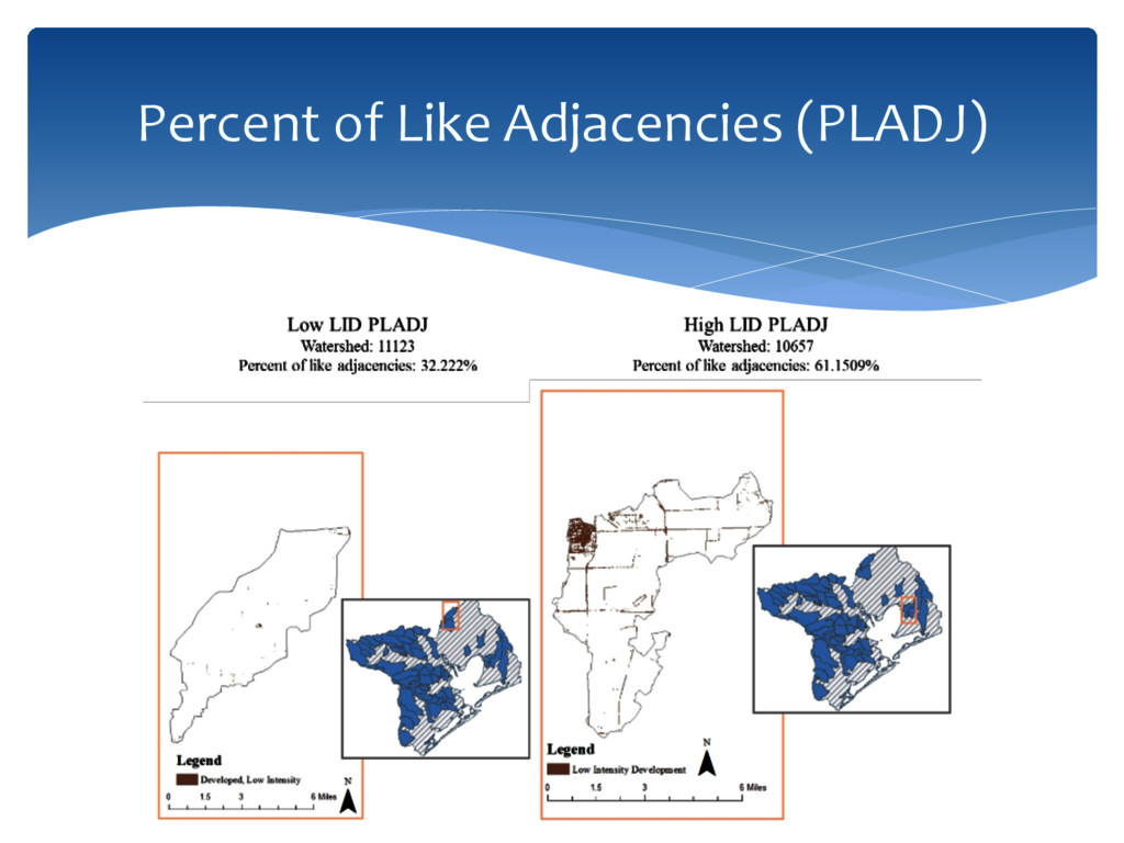
size, lower the phosphorus levels – greater patches means less edges and less of a way to enter stream. • Patch Density(+,p<0.001): high patch density means high phosphorus levels – more patches per area, greater the anthropogenic impacts (Carle et al., 2005). • Percent of Like adjacencies (-‐,p<0.05): higher PLADJ means more aggregated patches and therefore lower phosphorus levels. • Contiguity(-‐,p<0.1): The more continuous a patch is, the lower the phosphorus levels – more continuous patches means less fragmentation. Low Intensity Model Results
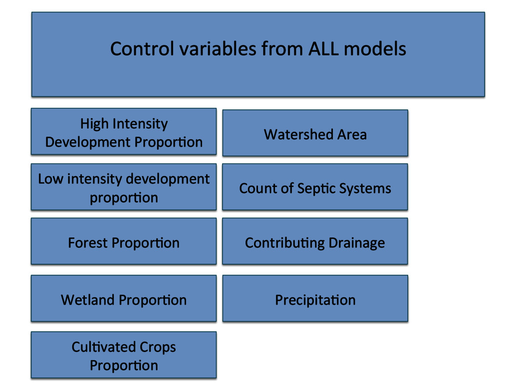
Count of SepLc Systems High Intensity Development ProporLon Low intensity development proporLon Wetland ProporLon Control variables from ALL models ContribuLng Drainage PrecipitaLon
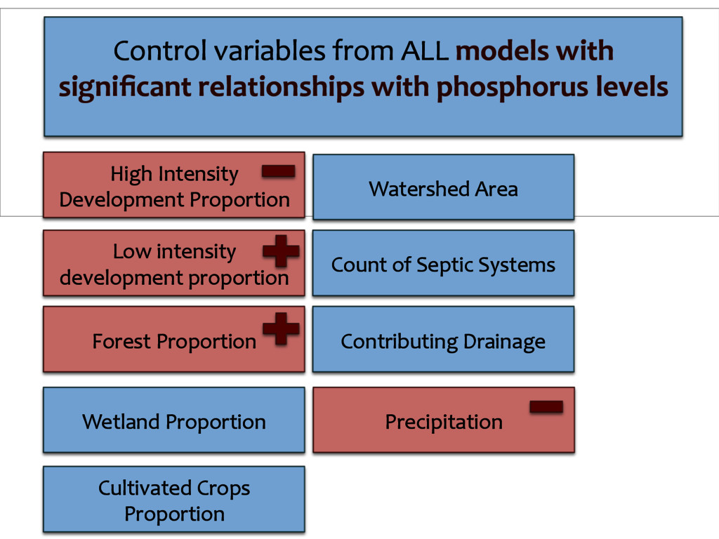
Count of Septic Systems High Intensity Development Proportion Low intensity development proportion Wetland Proportion Control variables from ALL models with significant relationships with phosphorus levels Contributing Drainage Precipitation
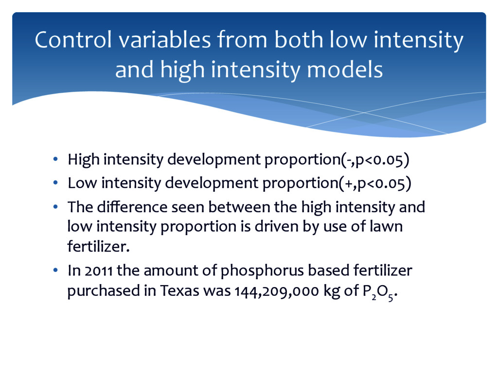
proportion(+,p<0.05) • The difference seen between the high intensity and low intensity proportion is driven by use of lawn fertilizer. • In 2011 the amount of phosphorus based fertilizer purchased in Texas was 144,209,000 kg of P2 O5 . Control variables from both low intensity and high intensity models
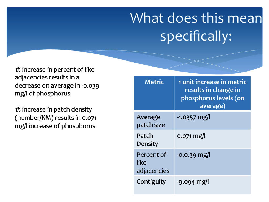
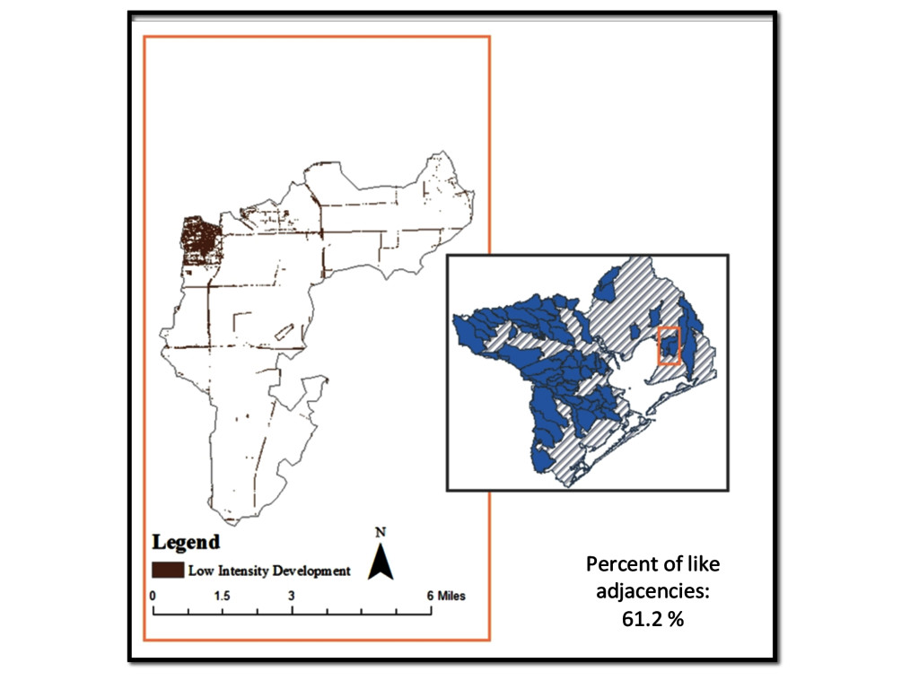
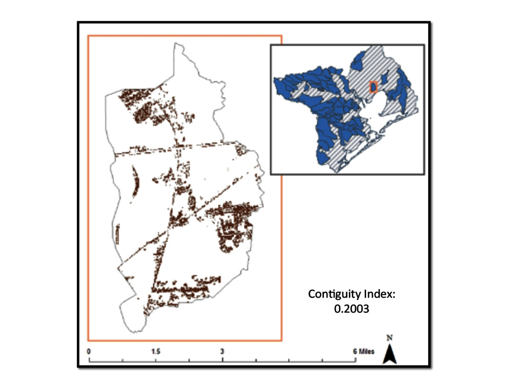
unit increase in metric results in change in phosphorus levels (on average) Average patch size -‐1.0357 mg/l Patch Density 0.071 mg/l Percent of like adjacencies -‐0.0.39 mg/l Contiguity -‐9.094 mg/l 1% increase in percent of like adjacencies results in a decrease on average in -‐0.039 mg/l of phosphorus. 1% increase in patch density (number/KM) results in 0.071 mg/l increase of phosphorus
owners can have a large impact on the level of phosphorus in the streams in the Galveston Bay Estuary. • Developing in a less fragmented manner has positive effects on the phosphorus levels. Concluding thoughts
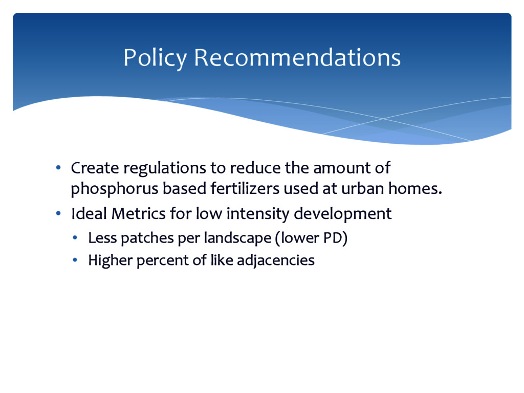
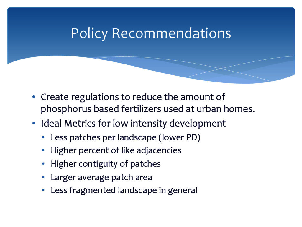
based fertilizers used at urban homes. • Ideal Metrics for low intensity development • Less patches per landscape (lower PD) • Higher percent of like adjacencies Policy Recommendations
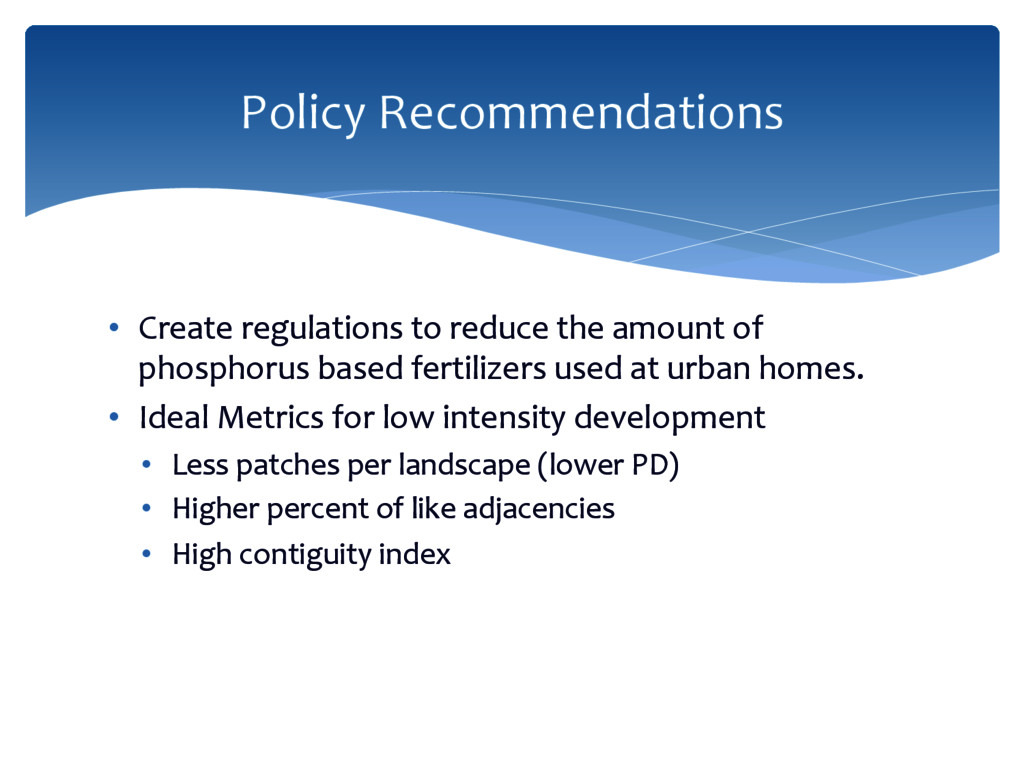
based fertilizers used at urban homes. • Ideal Metrics for low intensity development • Less patches per landscape (lower PD) • Higher percent of like adjacencies • High contiguity index Policy Recommendations
based fertilizers used at urban homes. • Ideal Metrics for low intensity development • Less patches per landscape (lower PD) • Higher percent of like adjacencies • Higher contiguity of patches • Larger average patch area • Less fragmented landscape in general Policy Recommendations
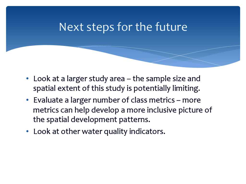
size and spatial extent of this study is potentially limiting. • Evaluate a larger number of class metrics – more metrics can help develop a more inclusive picture of the spatial development patterns. • Look at other water quality indicators. Next steps for the future
Dr. Samuel Brody, Dr. Wesley Highfield, Dr. Antonietta Quigg. • Research funded by Texas A&M Galveston 2 year competitive graduate merit fellowship. • Thank you to all my lab mates in the Center for Texas Beaches and Shores.
are shown to have a positive relationship with total phosphorus. For instance, Lee et al., (2009) showed that there was a positive relationship of TP with patch density and the study resulted in saying that the less fragmented but more complex the forest area is seems to preserve the water quality the best. This study went on to state that the degradation of water quality can come not only from increasing urban lands but also decreasing the quality of the remaining forests that have not been converted into urban lands (Lee et al., 2009). The summation of this is to say that highly fragmented forests do not function as a filter to provide the generally understood negative relationship with total phosphorus as is shown in numerous other studies . Forest Relationship
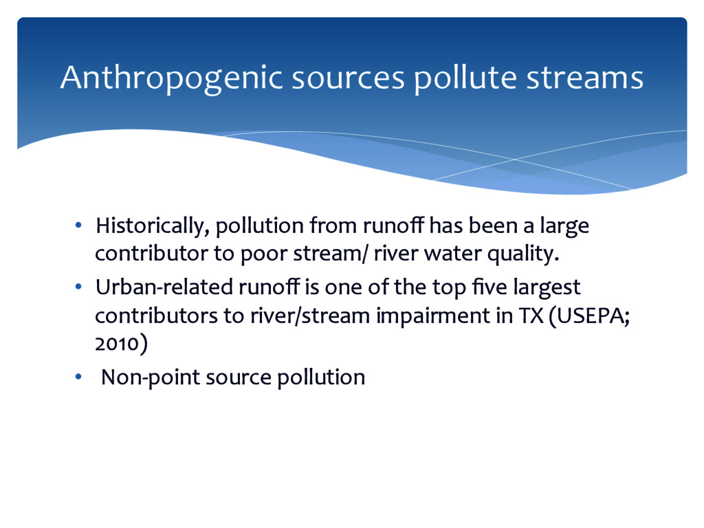
contributor to poor stream/ river water quality. • Urban-‐related runoff is one of the top five largest contributors to river/stream impairment in TX (USEPA; 2010) • Non-‐point source pollution Anthropogenic sources pollute streams
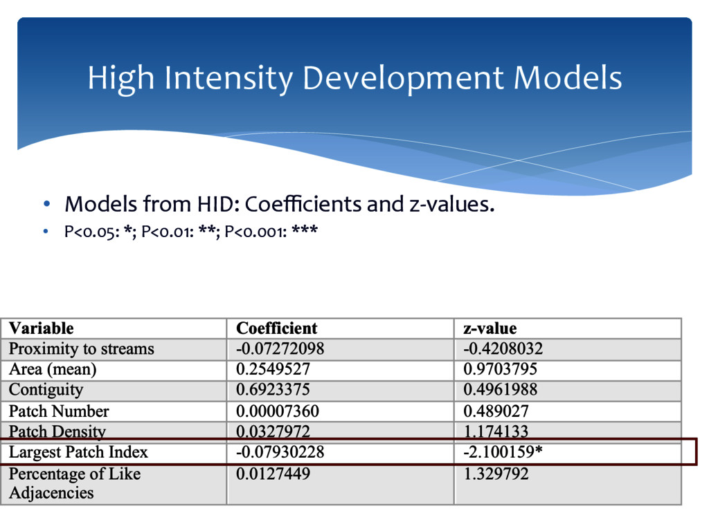
• There is 1 metric significant in HID model. • Multiple controls are significant with the most interesting being proportion of High intensity development (-‐) and proportion of low intensity development (+) Discussion of Results
is critical, as different spatial scales may show varying relationships between water quality indicators and urban land cover (Dietz and Clausen, 2008) • Small and large scale studies are done with differing levels of detail. Consideration 1: Different spatial scales
watershed can allow for more detail and potentially less assumptions. • Fewer watersheds can be used to study small details within a watershed, a greater number of samples are needed for statistical validity when looking at large-‐ scale correlations. Spatial Scales
important to control for. • Agriculture is positively correlated with total phosphorus. • Forest is negatively correlated with total phosphorus however, there can be a positive relationship depending on level of fragmentation • Wetlands retain a lot of input phosphorus and reduce the nutrient loading to the streams. Differing land cover types
and many metrics or vice versa • Precipitation • Seasonal variability • Other water quality variables (need to have a long and constant record of measurement) Consideration 2: How to measure phosphorus
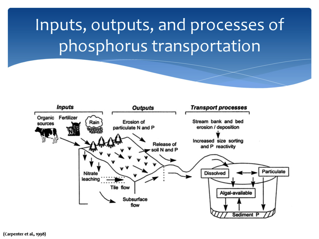
subsequently are contained in the runoff into streams/rivers. • In 2011 the amount of phosphorus based fertilizer was 144,209,000 kg (P2O5 which is 44% phosphorus) • Phosphorus is the limiting nutrient for algal growth and can lead to algal blooms. Phosphorus
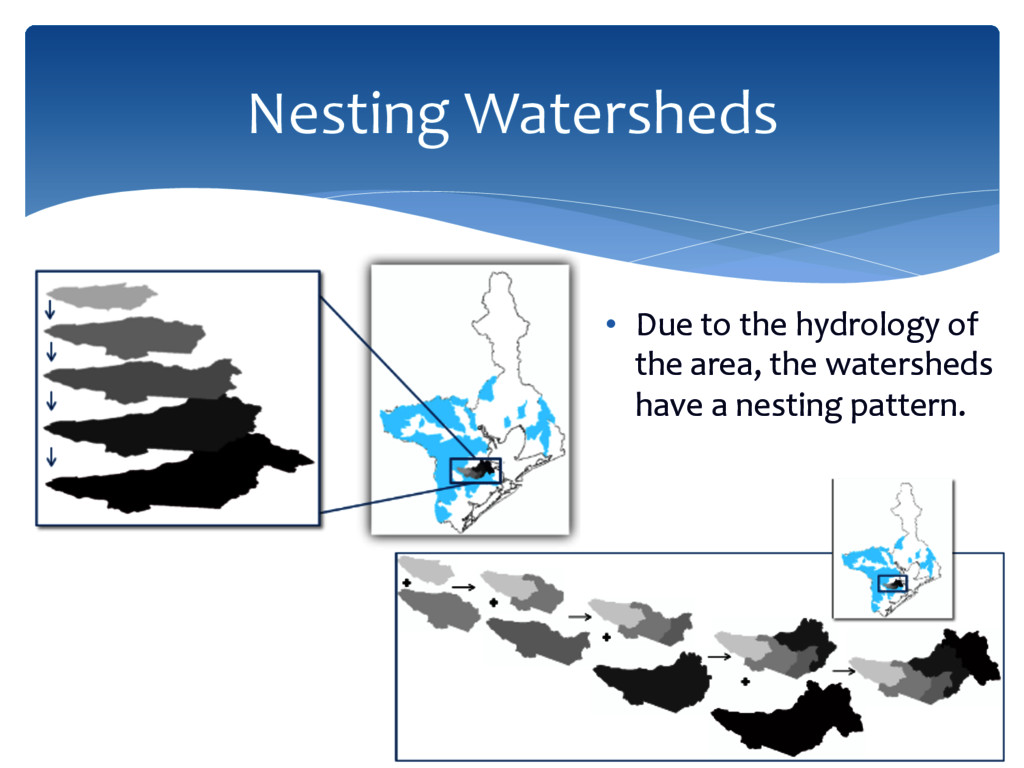
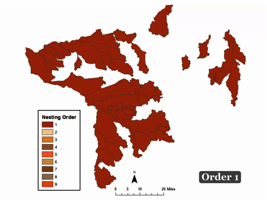
have an ecosystems approach. • Allows the area of the study watersheds to be controlled by hydrologic environment. Consideration 3: How to delineate watersheds
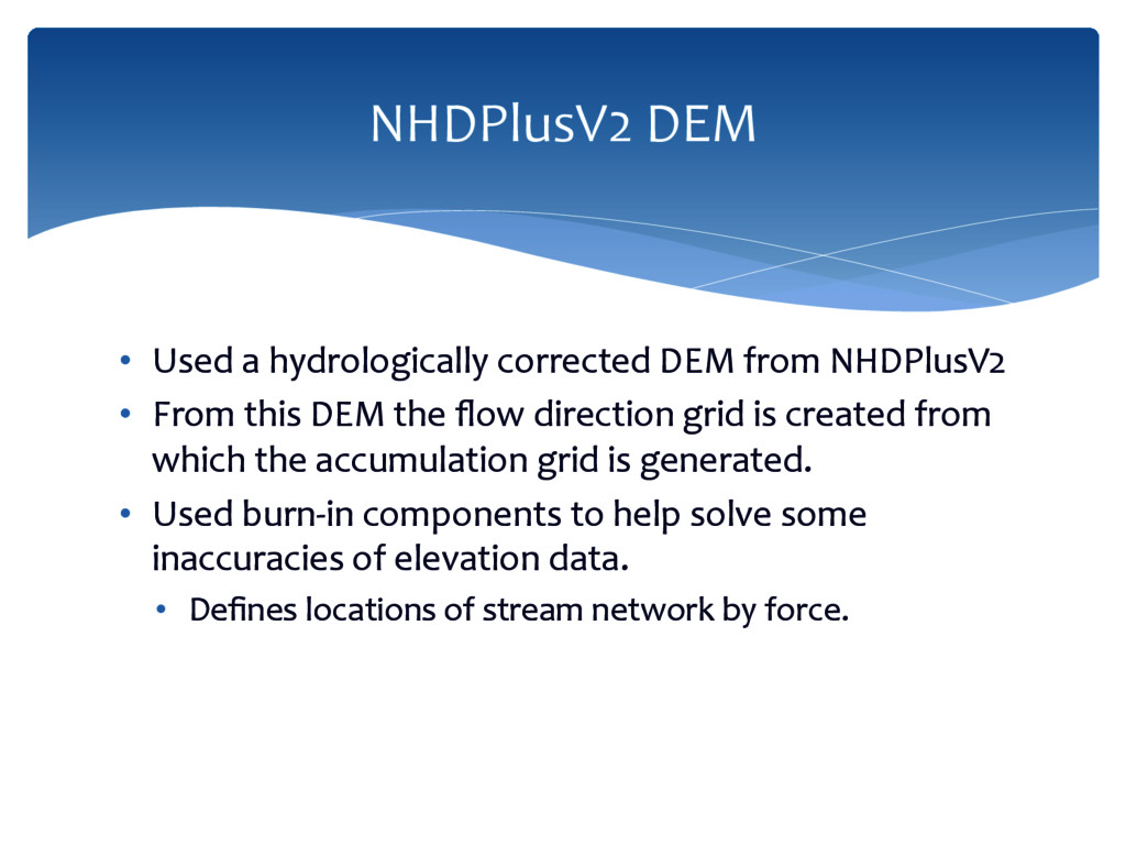
From this DEM the flow direction grid is created from which the accumulation grid is generated. • Used burn-‐in components to help solve some inaccuracies of elevation data. • Defines locations of stream network by force. NHDPlusV2 DEM
development vs low intensity development • General negative relationship between urban land cover and water quality. • Positive relationship between phosphorus and urban land (Tong and Chen, 2002 & Ahearn et al., 2005) Consideration 4: measuring and quantifying development in landscape
class i A = total landscape area (m) ni = number of patches in the landscape of class type i. aij = area of patchij ni = number of patches in landscape of patch type (class)i Cijr = contiguity value of r pixel r in patch ij V = sum of values in a 3x3 cell template Aij * = area of patch ij in terms of number of cell aij = area (m2 ) of patch ij A = total landscape area (m2). gij = number of like adjacencies (joins) between pixels of patch type (class) I based on the double-‐count method. gik = number of adjacencies (joins) between pixels of patch type (classes) I and k based on the double count method.
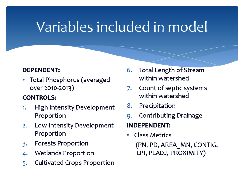
CONTROLS: 1. High Intensity Development Proportion 2. Low Intensity Development Proportion 3. Forests Proportion 4. Wetlands Proportion 5. Cultivated Crops Proportion 6. Total Length of Stream within watershed 7. Count of septic systems within watershed 8. Precipitation 9. Contributing Drainage INDEPENDENT: • Class Metrics (PN, PD, AREA_MN, CONTIG, LPI, PLADJ, PROXIMITY) Variables included in model
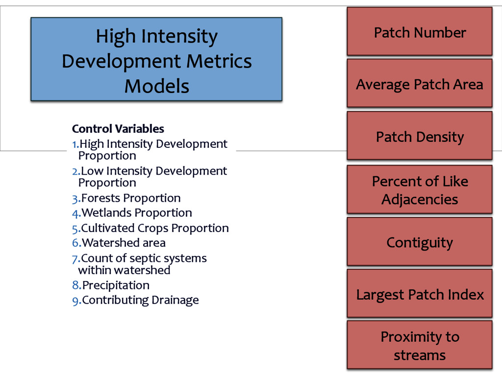
to streams Patch Number Average Patch Area Percent of Like Adjacencies High Intensity Development Metrics Models Control Variables 1. High Intensity Development Proportion 2. Low Intensity Development Proportion 3. Forests Proportion 4. Wetlands Proportion 5. Cultivated Crops Proportion 6. Watershed area 7. Count of septic systems within watershed 8. Precipitation 9. Contributing Drainage
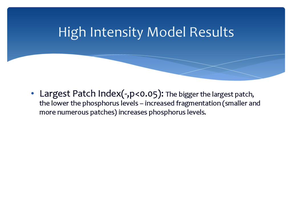
the lower the phosphorus levels – increased fragmentation (smaller and more numerous patches) increases phosphorus levels. High Intensity Model Results