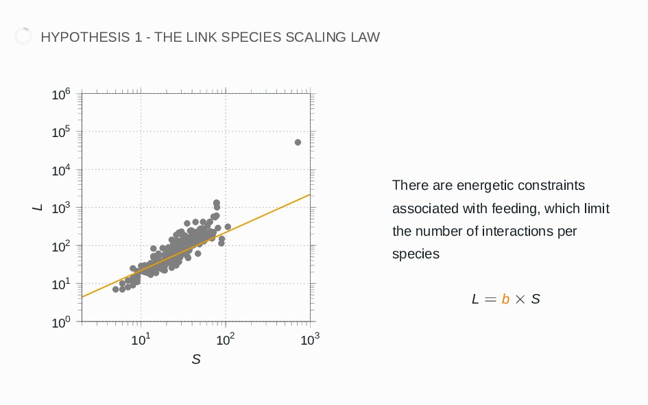
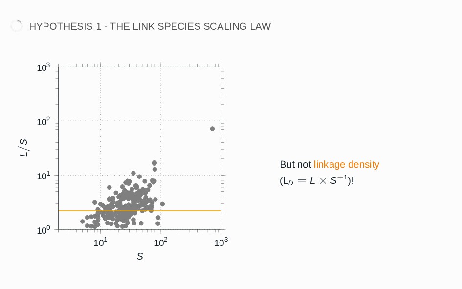
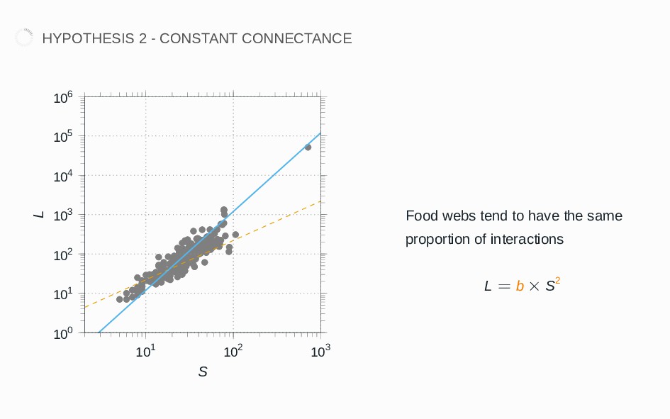
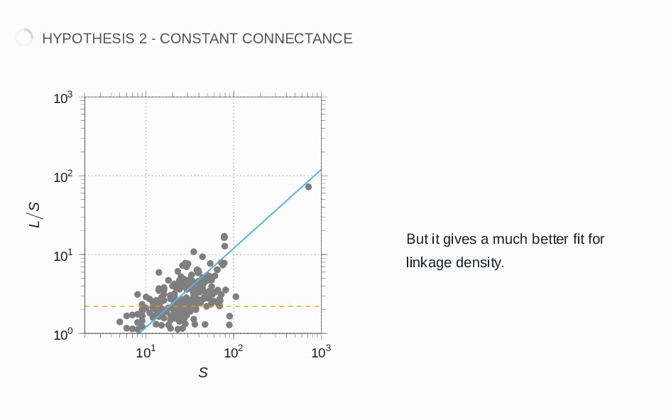
103 100 101 102 103 104 105 106 S L There are energetic constraints associated with feeding, which limit the number of interactions per species L = b × S
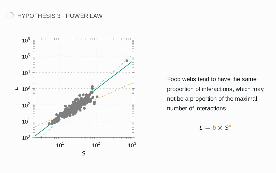
102 103 104 105 106 S L Food webs tend to have the same proportion of interactions, which may not be a proportion of the maximal number of interactions L = b × Sa
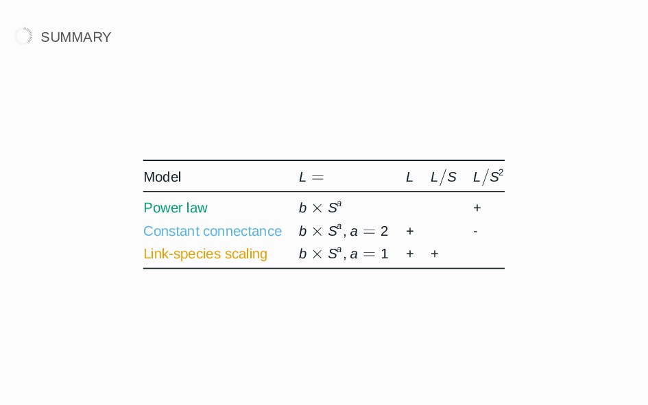
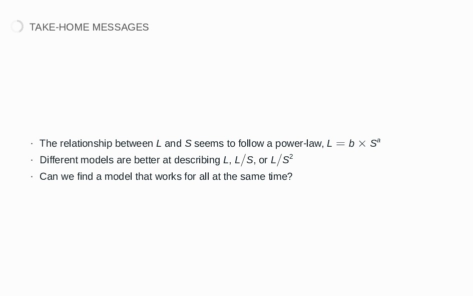
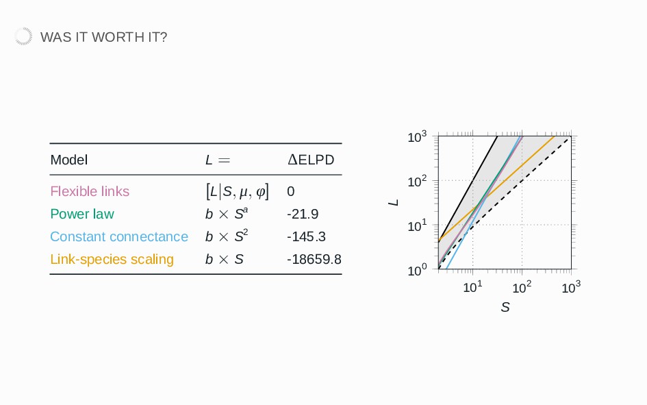
to follow a powerlaw, L = b × Sa · Different models are better at describing L, L/S, or L/S2 · Can we find a model that works for all at the same time?
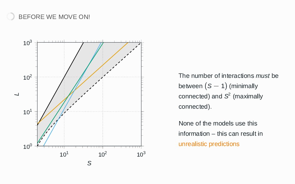
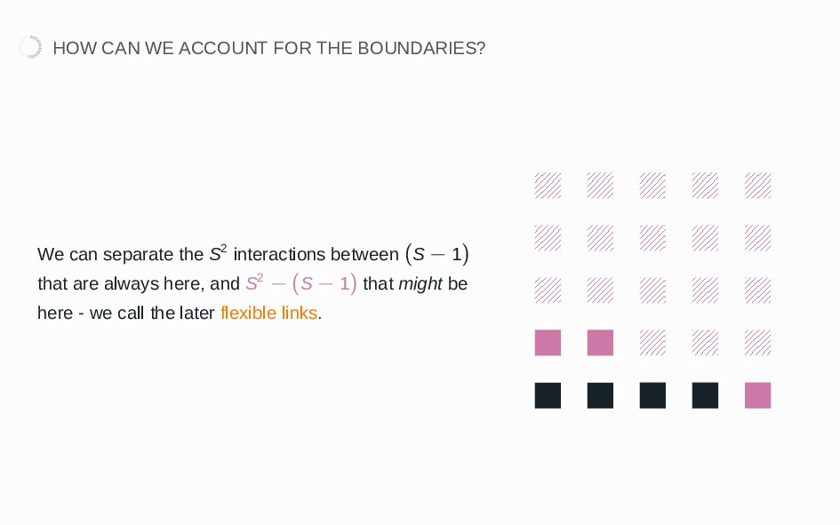
103 S L The number of interactions must be between (S − 1) (minimally connected) and S2 (maximally connected). None of the models use this information – this can result in unrealistic predictions
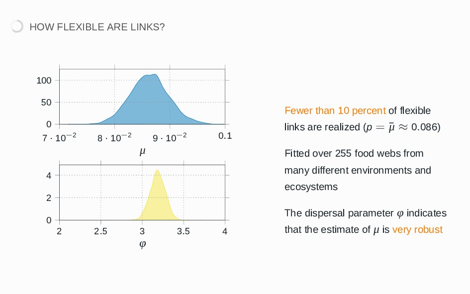
9 · 10−2 0.1 0 50 100 μ 2 2.5 3 3.5 4 0 2 4 φ Fewer than 10 percent of flexible links are realized (p = ¯ μ ≈ 0.086) Fitted over 255 food webs from many different environments and ecosystems The dispersal parameter φ indicates that the estimate of μ is very robust
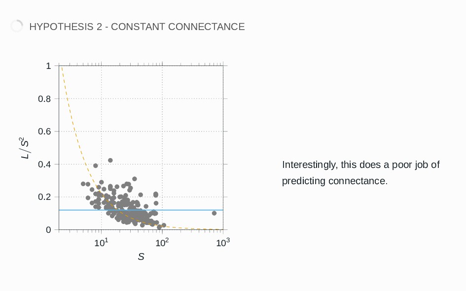
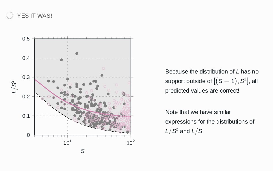
0.5 S L/S2 Because the distribution of L has no support outside of [(S − 1), S2], all predicted values are correct! Note that we have similar expressions for the distributions of L/S2 and L/S.
0.5 S L/S2 Because the distribution of L has no support outside of [(S − 1), S2], all predicted values are correct! Note that we have similar expressions for the distributions of L/S2 and L/S.
by looking at the proportion of flexible links · This has better fit than the previous models · This also always return predictions within the boundaries
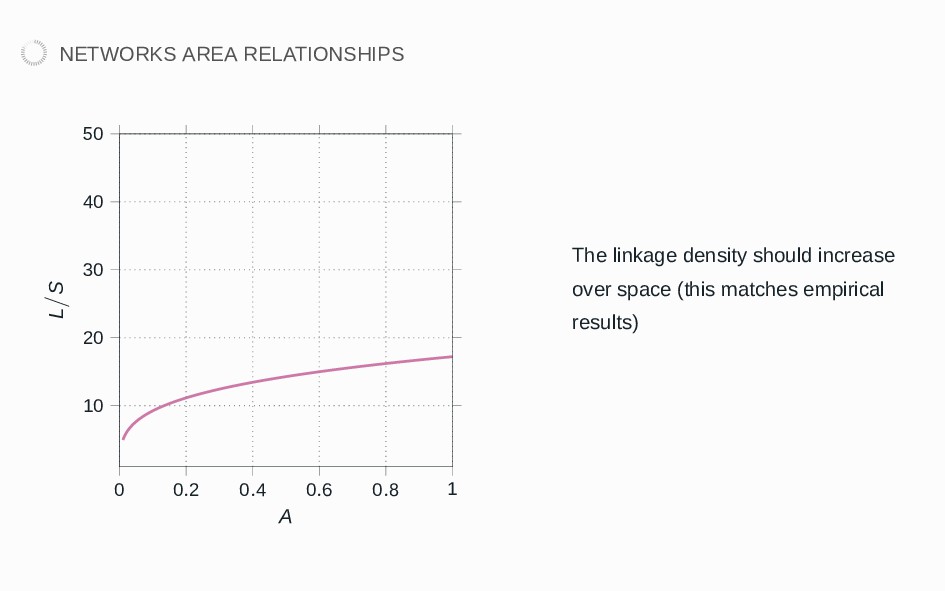
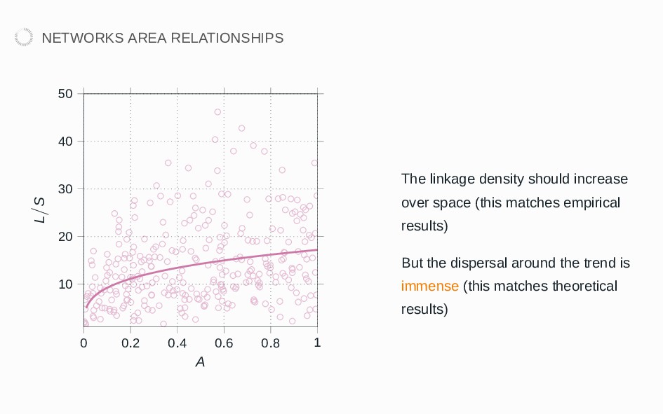
20 30 40 50 A L/S The linkage density should increase over space (this matches empirical results) But the dispersal around the trend is immense (this matches theoretical results)
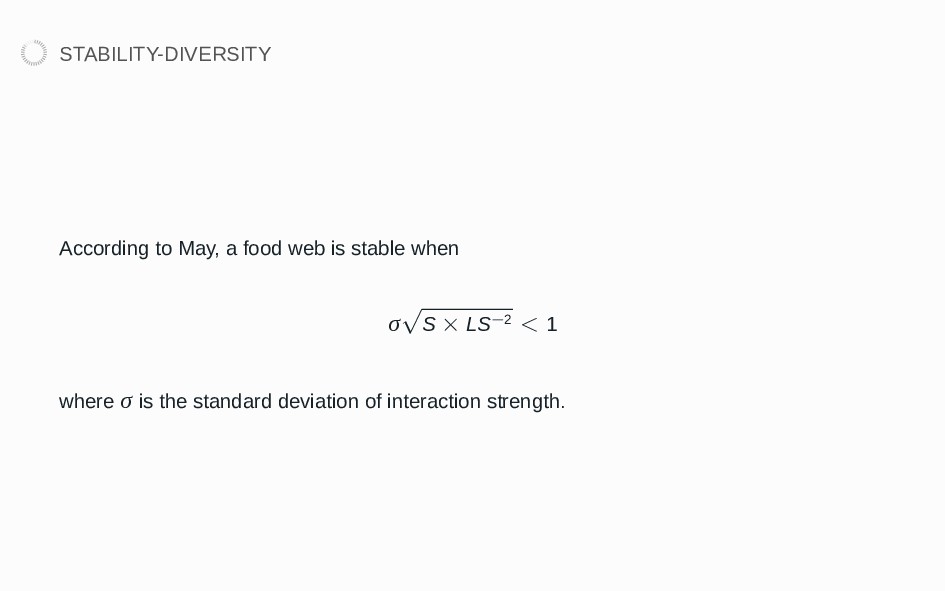
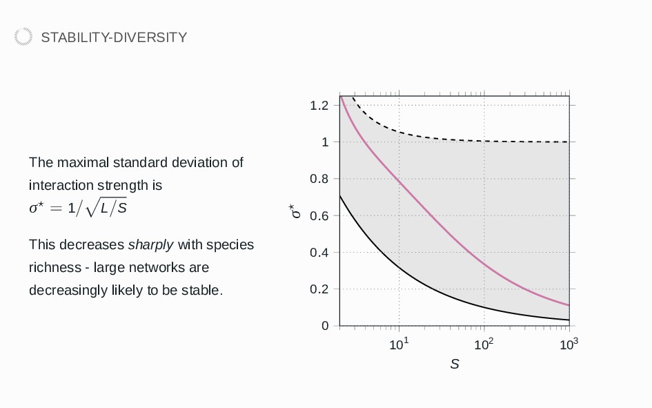
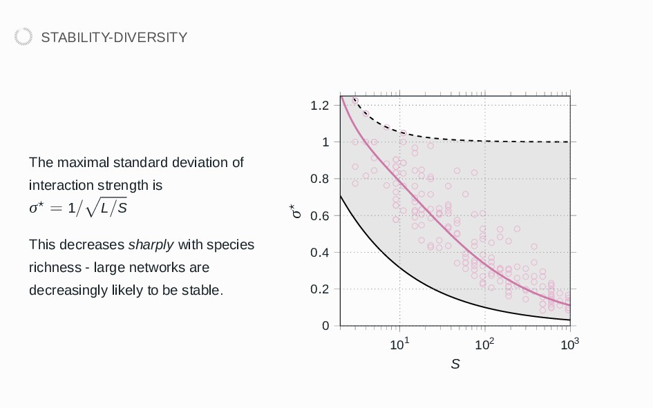
= 1/ √ L/S This decreases sharply with species richness large networks are decreasingly likely to be stable. 101 102 103 0 0.2 0.4 0.6 0.8 1 1.2 S σ⋆
= 1/ √ L/S This decreases sharply with species richness large networks are decreasingly likely to be stable. 101 102 103 0 0.2 0.4 0.6 0.8 1 1.2 S σ⋆
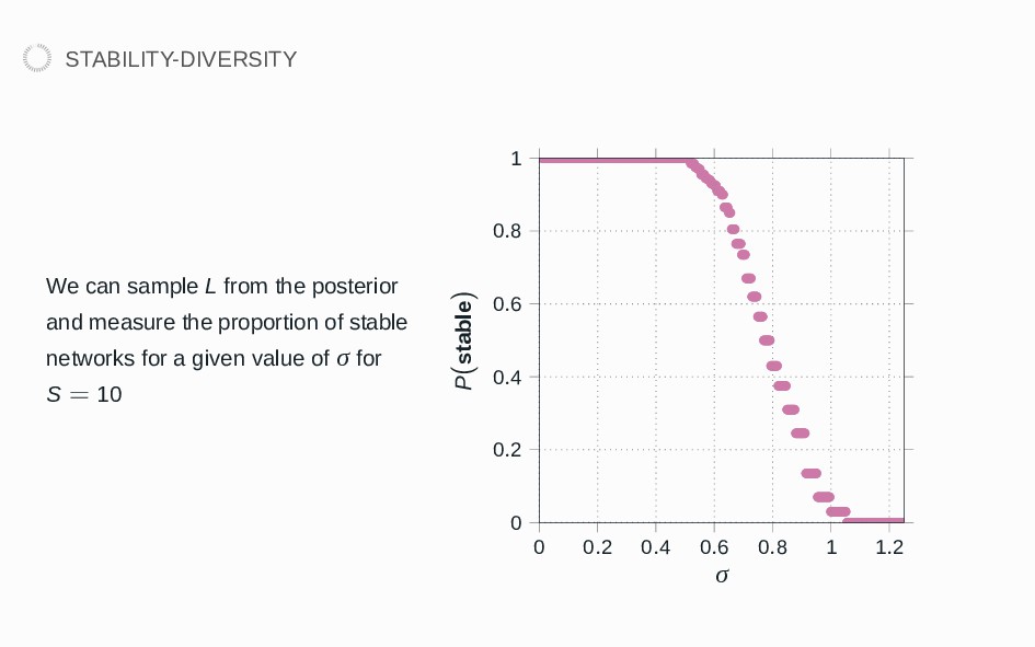
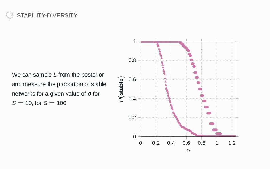
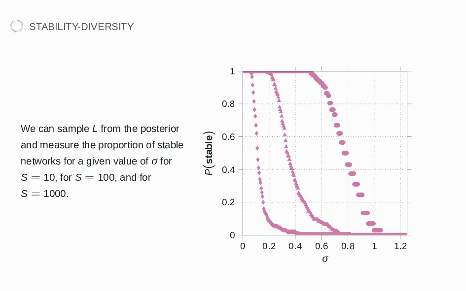
the proportion of stable networks for a given value of σ for S = 10, for S = 100, and for S = 1000. 0 0.2 0.4 0.6 0.8 1 1.2 0 0.2 0.4 0.6 0.8 1 σ P(stable)
![THANKS TO… Francis Banville ([email protected]) Andrew MacDonald ([email protected]) Revisiting the](https://files.speakerdeck.com/presentations/b75dde0825ff40ffb0ff689c480fd355/slide_2.jpg)
![THE FLEXIBLE LINKS MODEL IN PRACTICE [L|S, μ, φ] =](https://files.speakerdeck.com/presentations/b75dde0825ff40ffb0ff689c480fd355/slide_23.jpg)