What does Adam have to do with symplectic manifolds? - The geometry behind momentum methods in Machine Learning

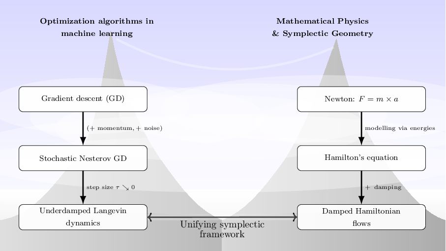
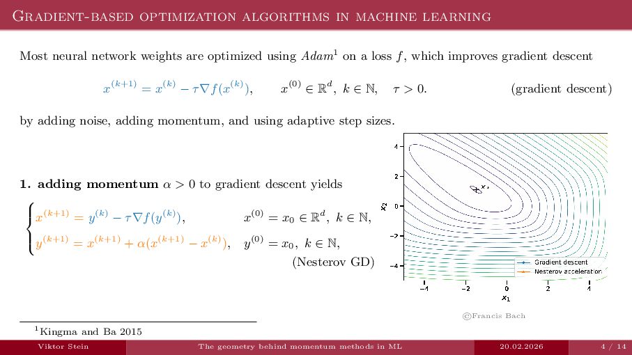
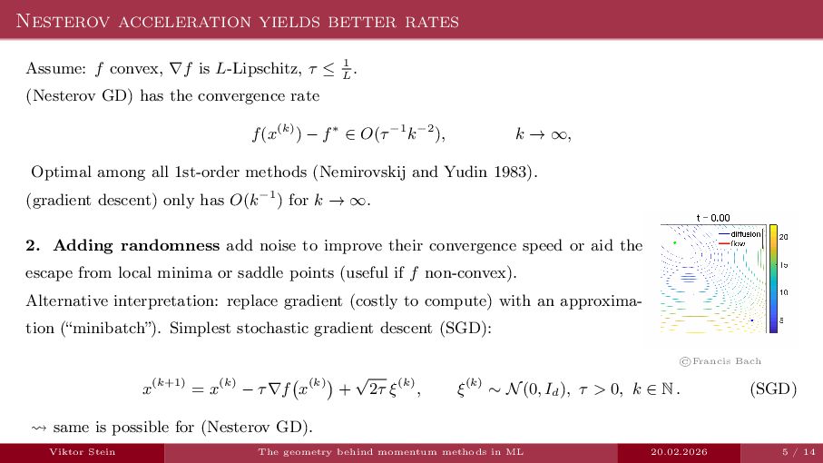
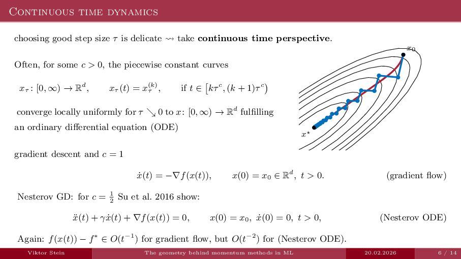
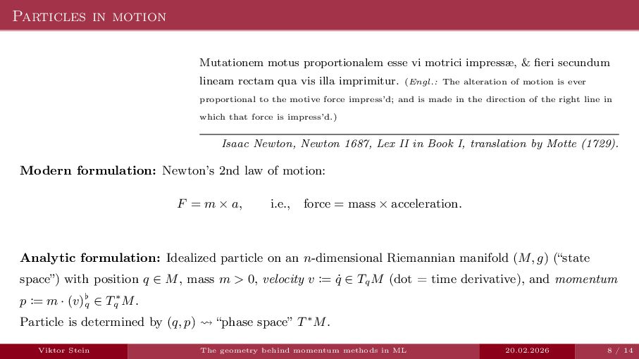
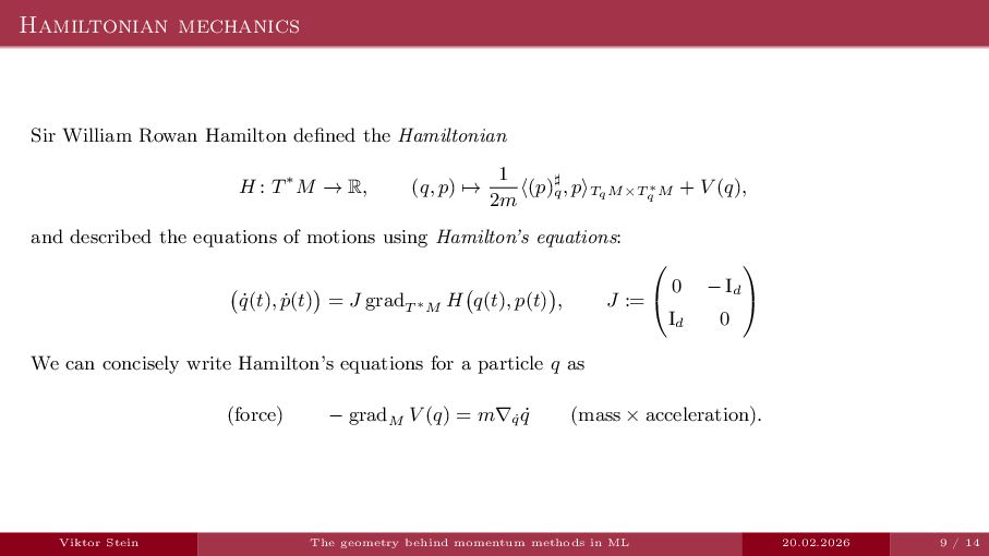
Gradient-based optimization algorithms are indispensable for most modern machine learning applications, since they are used to train convolutional neural networks (CNNs) for image classification or transformers for natural language processing. Often, the weights are optimized using the Adam algorithm, a momentum-based modification of gradient descent. In the vanishing step-size limit, these momentum-based algorithms can be described as second-order damped dynamics with a time-dependent Hamiltonian interpretation.
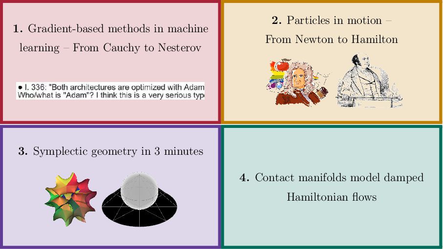
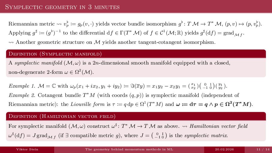
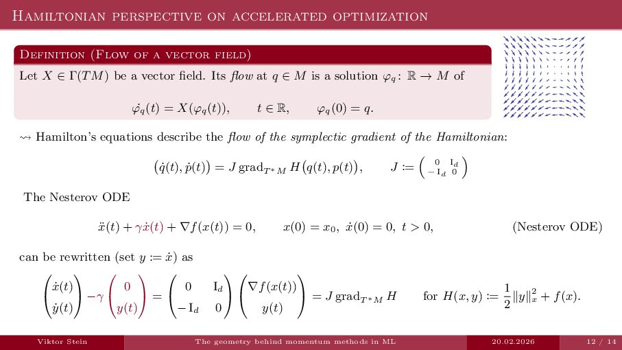
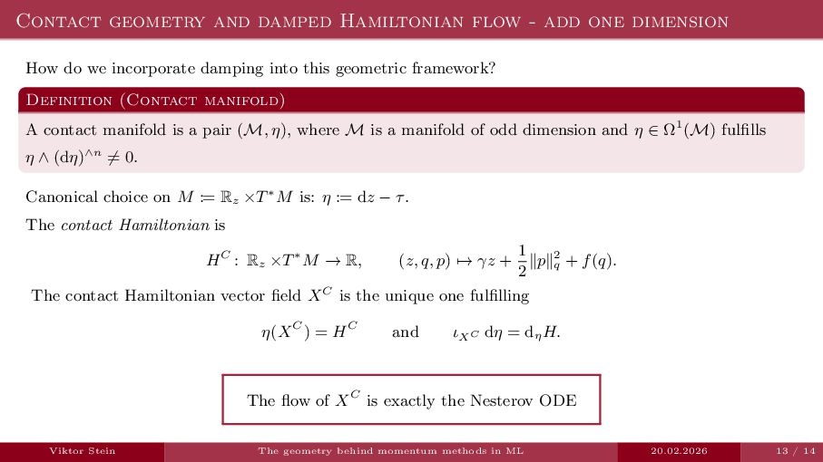
In this talk, I will gently introduce the contact geometry behind time-dependent Hamiltonian systems and show how viewing momentum-based methods in machine learning through this geometric lens can help elucidate their properties.

Transcript

1. What does Adam have to do with symplectic manifolds? The geometry behind momentum methods in machine learning Viktor Stein, Technical University of Berlin 14th BMS Student Conference 20.02.2026
2. Math as mountain Landscape NYT "The singular mind of Terry Tao" (26.07.15) “I have often heard mathematics described in terms of a land- scape shrouded in fog and mist. At first, there is nothing to see; then, as the mist lowers, you begin to observe isolated peaks. A little later, when the mist is lower still, you start to see connec- tions between the peaks. When [...] the fog dissipates almost entirely, [...] you finally begin to see the cities and roads at the bottom of the landscape, in between all the peaks. That’s where some really interesting stuff happens. – Terry Tao in Do Not Erase by Jessica Wynne (Princeton University Press, 2021)” Viktor Stein The geometry behind momentum methods in ML 20.02.2026 2 / 14
3. Optimization algorithms in machine learning Mathematical Physics & Symplectic Geometry Gradient descent (GD) Stochastic Nesterov GD Underdamped Langevin dynamics (+ momentum, + noise) step size τ ↘ 0 Newton: F = m × a Hamilton’s equation Damped Hamiltonian flows modelling via energies + damping Unifying symplectic framework
4. Gradient-based optimization algorithms in machine learning Most neural network weights are optimized using Adam1 on a loss f, which improves gradient descent x(k+1) = x(k) − τ∇f(x(k)), x(0) ∈ Rd, k ∈ N, τ > 0. (gradient descent) by adding noise, adding momentum, and using adaptive step sizes. 1. adding momentum α > 0 to gradient descent yields      x(k+1) = y(k) − τ∇f(y(k)), x(0) = x0 ∈ Rd, k ∈ N, y(k+1) = x(k+1) + α(x(k+1) − x(k)), y(0) = x0 , k ∈ N, (Nesterov GD) ©Francis Bach 1Kingma and Ba 2015 Viktor Stein The geometry behind momentum methods in ML 20.02.2026 4 / 14
5. Nesterov acceleration yields better rates Assume: f convex, ∇f is L-Lipschitz, τ ≤ 1 L . (Nesterov GD) has the convergence rate f(x(k)) − f∗ ∈ O(τ−1k−2), k → ∞, Optimal among all 1st-order methods (Nemirovskij and Yudin 1983). (gradient descent) only has O(k−1) for k → ∞. 2. Adding randomness add noise to improve their convergence speed or aid the escape from local minima or saddle points (useful if f non-convex). Alternative interpretation: replace gradient (costly to compute) with an approxima- tion (“minibatch”). Simplest stochastic gradient descent (SGD): ©Francis Bach x(k+1) = x(k) − τ∇f x(k) + √ 2τ ξ(k), ξ(k) ∼ N(0, Id ), τ > 0, k ∈ N . (SGD) ⇝ same is possible for (Nesterov GD). Viktor Stein The geometry behind momentum methods in ML 20.02.2026 5 / 14
6. Continuous time dynamics choosing good step size τ is delicate ⇝ take continuous time perspective. Often, for some c > 0, the piecewise constant curves xτ : [0, ∞) → Rd, xτ (t) = x(k) τ , if t ∈ kτc, (k + 1)τc converge locally uniformly for τ ↘ 0 to x: [0, ∞) → Rd fulfilling an ordinary differential equation (ODE) x0 x⋆ gradient descent and c = 1 ˙ x(t) = −∇f(x(t)), x(0) = x0 ∈ Rd, t > 0. (gradient flow) Nesterov GD: for c = 1 2 Su et al. 2016 show: ¨ x(t) + γ ˙ x(t) + ∇f(x(t)) = 0, x(0) = x0 , ˙ x(0) = 0, t > 0, (Nesterov ODE) Again: f(x(t)) − f∗ ∈ O(t−1) for gradient flow, but O(t−2) for (Nesterov ODE). Viktor Stein The geometry behind momentum methods in ML 20.02.2026 6 / 14
7. 1. Gradient-based methods in machine learning – From Cauchy to Nesterov 2. Particles in motion – From Newton to Hamilton 3. Symplectic geometry in 3 minutes 4. Contact manifolds model damped Hamiltonian flows
8. Particles in motion Mutationem motus proportionalem esse vi motrici impressæ, & fieri secundum lineam rectam qua vis illa imprimitur. (Engl.: The alteration of motion is ever proportional to the motive force impress’d; and is made in the direction of the right line in which that force is impress’d.) Isaac Newton, Newton 1687, Lex II in Book I, translation by Motte (1729). Modern formulation: Newton’s 2nd law of motion: F = m × a, i.e., force = mass × acceleration. Analytic formulation: Idealized particle on an n-dimensional Riemannian manifold (M, g) (“state space”) with position q ∈ M, mass m > 0, velocity v := ˙ q ∈ Tq M (dot = time derivative), and momentum p := m · (v)♭ q ∈ T∗ q M. Particle is determined by (q, p) ⇝ “phase space” T∗M. Viktor Stein The geometry behind momentum methods in ML 20.02.2026 8 / 14
9. Hamiltonian mechanics Sir William Rowan Hamilton defined the Hamiltonian H : T∗M → R, (q, p) → 1 2m ⟨(p)♯ q , p⟩TqM×T ∗ q M + V (q), and described the equations of motions using Hamilton’s equations: ˙ q(t), ˙ p(t) = J gradT ∗M H q(t), p(t) , J :=   0 − Id Id 0   We can concisely write Hamilton’s equations for a particle q as (force) − gradM V (q) = m∇˙ q ˙ q (mass × acceleration). Viktor Stein The geometry behind momentum methods in ML 20.02.2026 9 / 14
10. 1. Gradient-based methods in machine learning – From Cauchy to Nesterov 2. Particles in motion – From Newton to Hamilton 3. Symplectic geometry in 3 minutes 4. Contact manifolds model damped Hamiltonian flows
11. Symplectic geometry in 3 minutes Riemannian metric ⇝ v♭ p := gp (v, ·) yields vector bundle isomorphism g♭ : T M → T∗ M, (p, v) → (p, v♭ p ). Applying g♯ := (g♭)−1 to the differential df ∈ Γ(T∗ M) of f ∈ C1(M; R) yields g♯(df) = gradM f . ⇝ Another geometric structure on M yields another tangent-cotangent isomorphism. Definition (Symplectic manifold) A symplectic manifold (M, ω) is a 2n-dimensional smooth manifold equipped with a closed, non-degenerate 2-form ω ∈ Ω2(M). Example 1. M = C with ωp (x1 + ix2 , y1 + iy2 ) := ℑ(xy) = x1 y2 − x2 y1 = ( x1 x2 ) 0 1 −1 0 ( y1 y2 ). Example 2. Cotangent bundle T∗M (with coords (q, p)) is symplectic manifold (independent of Riemannian metric): the Liouville form is τ := q dp ∈ Ω1(T∗M) and ω := dτ = q ∧ p ∈ Ω2(T ∗M). Definition (Hamiltonian vector field) For symplectic manifold (M, ω) construct ω♯ : T∗ M → T M as above. ⇝ Hamiltonian vector field ω♯(df) = J gradM f (if ∃ compatible metric g), where J = 0 I − I 0 is the symplectic matrix. Viktor Stein The geometry behind momentum methods in ML 20.02.2026 11 / 14
12. Hamiltonian perspective on accelerated optimization Definition (Flow of a vector field) Let X ∈ Γ(TM) be a vector field. Its flow at q ∈ M is a solution φq : R → M of ˙ φq (t) = X(φq (t)), t ∈ R, φq (0) = q. ⇝ Hamilton’s equations describe the flow of the symplectic gradient of the Hamiltonian: ˙ q(t), ˙ p(t) = J gradT ∗M H q(t), p(t) , J := 0 Id − Id 0 The Nesterov ODE ¨ x(t) + γ ˙ x(t) + ∇f(x(t)) = 0, x(0) = x0 , ˙ x(0) = 0, t > 0, (Nesterov ODE) can be rewritten (set y := ˙ x) as   ˙ x(t) ˙ y(t)   −γ   0 y(t)   =   0 Id − Id 0     ∇f(x(t)) y(t)   = J gradT ∗M H for H(x, y) := 1 2 ∥y∥2 x + f(x). Viktor Stein The geometry behind momentum methods in ML 20.02.2026 12 / 14
13. Contact geometry and damped Hamiltonian flow - add one dimension How do we incorporate damping into this geometric framework? Definition (Contact manifold) A contact manifold is a pair (M, η), where M is a manifold of odd dimension and η ∈ Ω1(M) fulfills η ∧ (dη)∧n ̸= 0. Canonical choice on M := Rz ×T∗M is: η := dz − τ. The contact Hamiltonian is HC : Rz ×T∗M → R, (z, q, p) → γz + 1 2 ∥p∥2 q + f(q). The contact Hamiltonian vector field XC is the unique one fulfilling η(XC ) = HC and ιXC dη = dη H. The flow of XC is exactly the Nesterov ODE Viktor Stein The geometry behind momentum methods in ML 20.02.2026 13 / 14
14. Thank you for your attention! I am happy to take any questions. Viktor Stein The geometry behind momentum methods in ML 20.02.2026 14 / 14
15. Bibliography [1] D. Kingma and J. Ba, “Adam: A method for stochastic optimization,” in International Conference on Learning Representations, Dec. 2015. [2] Nemirovskij and D. B. Yudin, Problem complexity and method efficiency in optimization. Wiley-Interscience, 1983. [3] W. Su, S. Boyd, and E. J. Candes, “A differential equation for modeling Nesterov’s accelerated gradient method: Theory and insights,” Journal of Machine Learning Research, vol. 17, no. 153, pp. 1–43, 2016. [4] I. Newton, Philosophiæ naturalis principia mathematica. Jussu Societatis Regiæ ac Typis Josephi Streater. Londini., 1687, First edition (Latin). Viktor Stein The geometry behind momentum methods in ML 20.02.2026 1 / 1