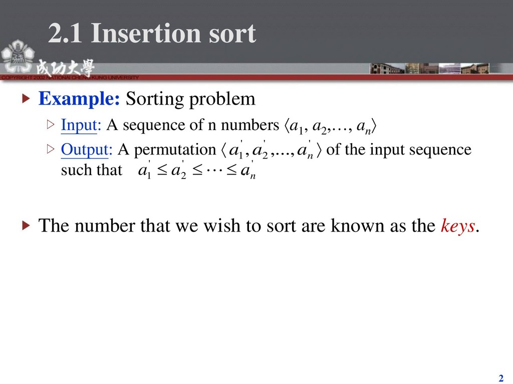
Upgrade to Pro — share decks privately, control downloads, hide ads and more …

[CS Foundation] Algorithm - 2 - Getting started

[CS Foundation] Algorithm - 2 - Getting started

x-village

August 06, 2018
Tweet

More Decks by x-village

Other Decks in Programming

Transcript

  1. 2 2.1 Insertion sort Example: Sorting problem Input: A sequence

    of n numbers a1 , a2 ,…, an  Output: A permutation   of the input sequence such that . The number that we wish to sort are known as the keys. ' ' 2 ' 1 ,..., , n a a a ' ' 2 ' 1 n a a a    
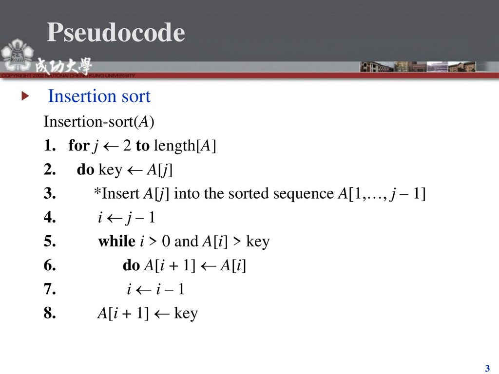
  2. 3 Pseudocode Insertion sort Insertion-sort(A) 1. for j  2

    to length[A] 2. do key  A[j] 3. *Insert A[j] into the sorted sequence A[1,…, j – 1] 4. i  j – 1 5. while i > 0 and A[i] > key 6. do A[i + 1]  A[i] 7. i  i – 1 8. A[i + 1]  key
  3. 4 The operation of Insertion-Sort 1 2 3 4 5

    6 5 2 4 6 1 3 1 2 3 4 5 6 2 5 4 6 1 3 1 2 3 4 5 6 2 4 5 6 1 3 1 2 3 4 5 6 2 4 5 6 1 3 1 2 3 4 5 6 1 2 4 5 6 3 1 2 3 4 5 6 1 2 3 4 5 6 (a) (c) (e) (b) (d) (f)
  4. 5 Sorted in place: The numbers are rearranged within the

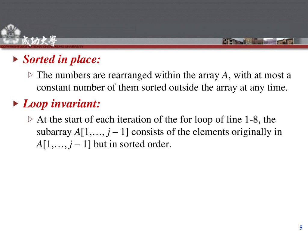
    array A, with at most a constant number of them sorted outside the array at any time. Loop invariant: At the start of each iteration of the for loop of line 1-8, the subarray A[1,…, j – 1] consists of the elements originally in A[1,…, j – 1] but in sorted order.
  5. 6 2.2 Analyzing algorithms Analyzing an algorithm has come to

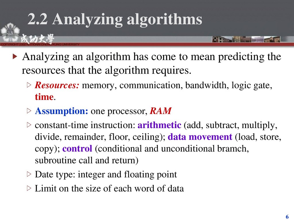
    mean predicting the resources that the algorithm requires. Resources: memory, communication, bandwidth, logic gate, time. Assumption: one processor, RAM constant-time instruction: arithmetic (add, subtract, multiply, divide, remainder, floor, ceiling); data movement (load, store, copy); control (conditional and unconditional bramch, subroutine call and return) Date type: integer and floating point Limit on the size of each word of data
  6. 7 2.2 Analyzing algorithms The best notion for input size

    depends on the problem being studied. The running time of an algorithm on a particular input is the number of primitive operations or “steps” executed. It is convenient to define the notion of step so that it is as machine-independent as possible.
  7. 8 Analysis of insertion sort Insertion-sort(A) 1. for j 

    2 to length[A] 2. do key  A[j] 3. *Insert A[j] into the sorted sequence A[1,…, j – 1] 4. i  j – 1 5. while i > 0 and A[i] > key 6. do A[i + 1]  A[i] 7. i  i – 1 8. A[i + 1]  key tj : the number of times the while loop test in line 5 is executed for the value of j. cost c1 c2 0 c4 c5 c6 c7 c8 cost n n – 1 n – 1 n – 1   n j j t 2    n j j t 2 ) 1 (    n j j t 2 ) 1 (
  8. 9 Analysis of insertion sort The running time T(n) =

    c1 n + c2 (n – 1) + c4 (n – 1) + c5 + c6 + c7 + c8 (n – 1) tj = 1, for j = 2, 3,…, n: Linear function on n T(n) = c1 n + c2 (n – 1) + c4 (n – 1) + c5 (n – 1) + c8 (n – 1) = (c1 + c2 + c4 + c5 + c8 )n – (c2 + c4 + c5 + c8 )   n j j t 2    n j j t 2 ) 1 (    n j j t 2 ) 1 (
  9. 10 Analysis of insertion sort tj = j, for j

    = 2, 3,…, n: Quadratic function on n T(n) = c1 n + c2 (n – 1) + c4 (n – 1) + c5 + c6 + c7 + c8 (n – 1) = n2 – (c1 + c2 + c4 + + c8 )n – (c2 + c4 + c5 + c8 ) ) 1 2 ) 1 ( (   n n ) 2 ) 1 ( (  n n ) 2 ) 1 ( (  n n ) 2 ( 7 6 5 c c c   ) 2 ( 7 6 5 c c c  
  10. 11 Worst-case and average-case analysis Usually, we concentrate on finding

    only on the worst- case running time. Reason: It is an upper bound on the running time. The worst case occurs fair often. The average case is often as bad as the worst case. For example, the insertion sort. Again, quadratic function.
  11. 12 Order of growth In some particular cases, we shall

    be interested in average-case, or expect running time of an algorithm. It is the rate of growth, or order of growth, of the running time that really interests us.
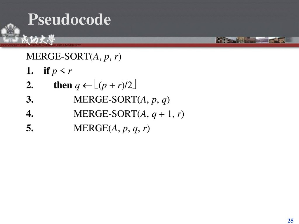
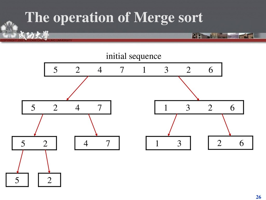
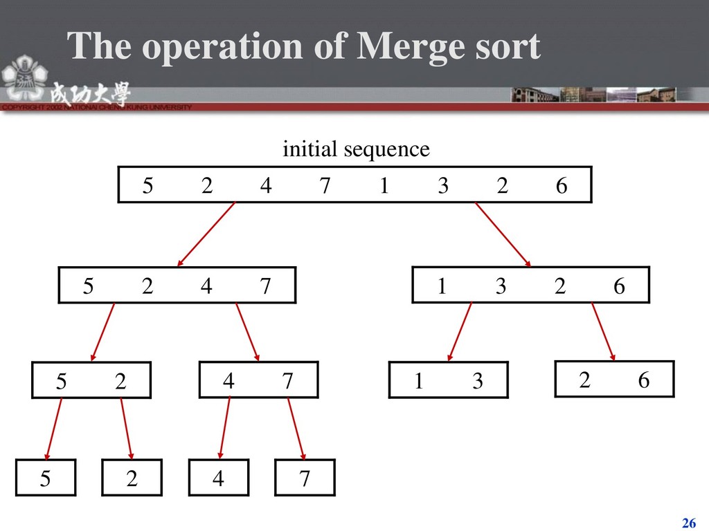
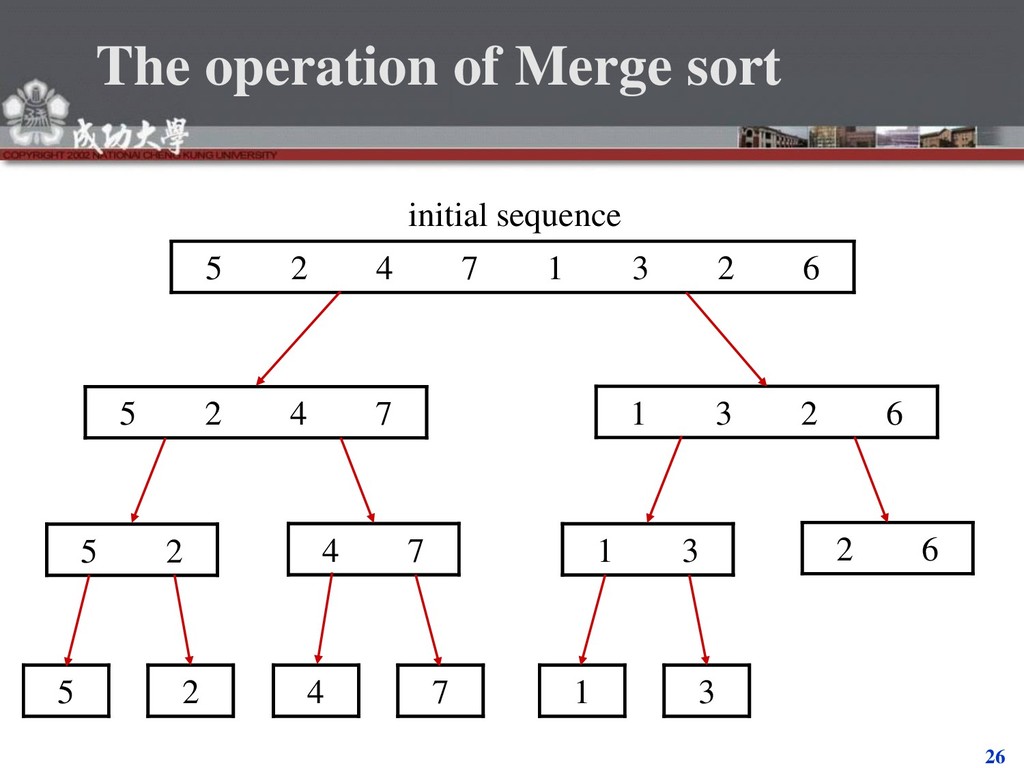
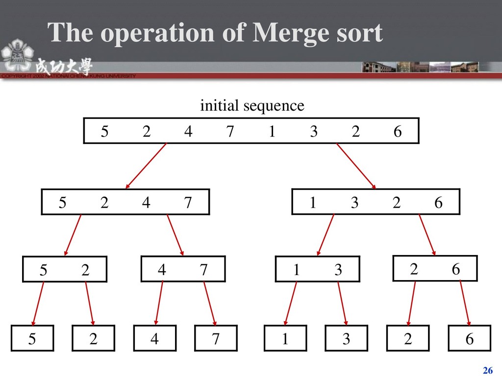
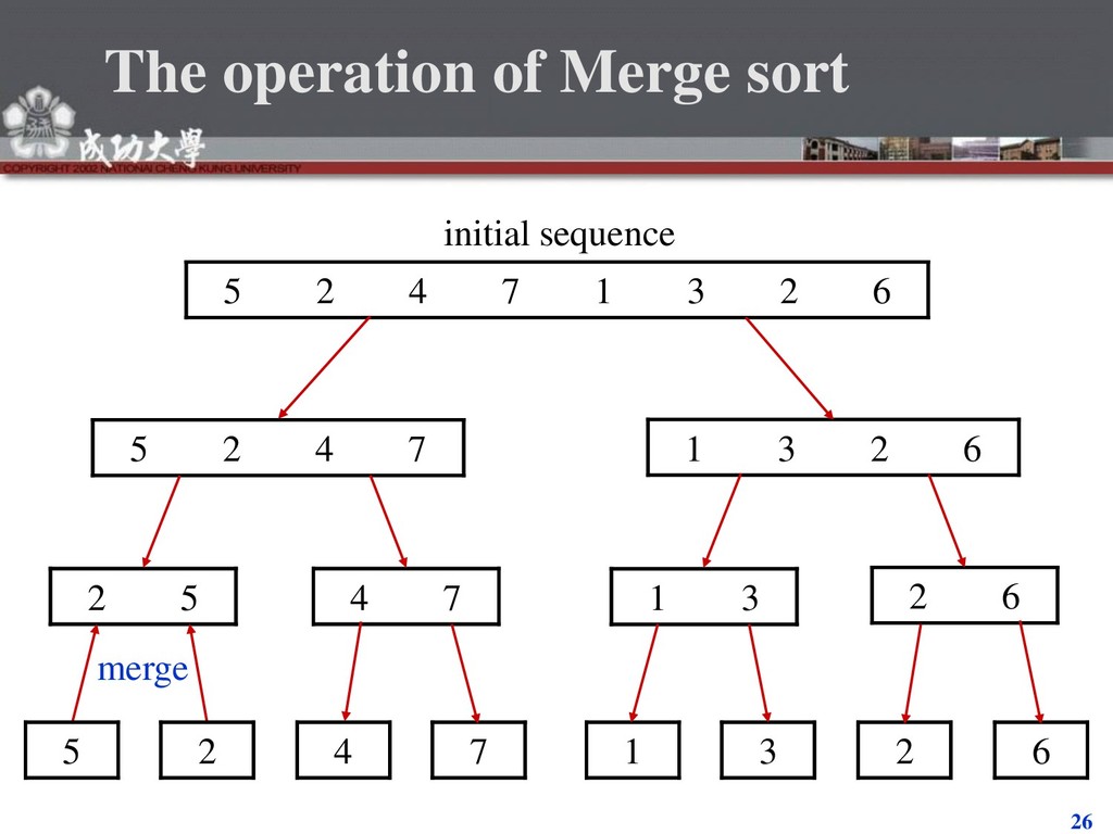
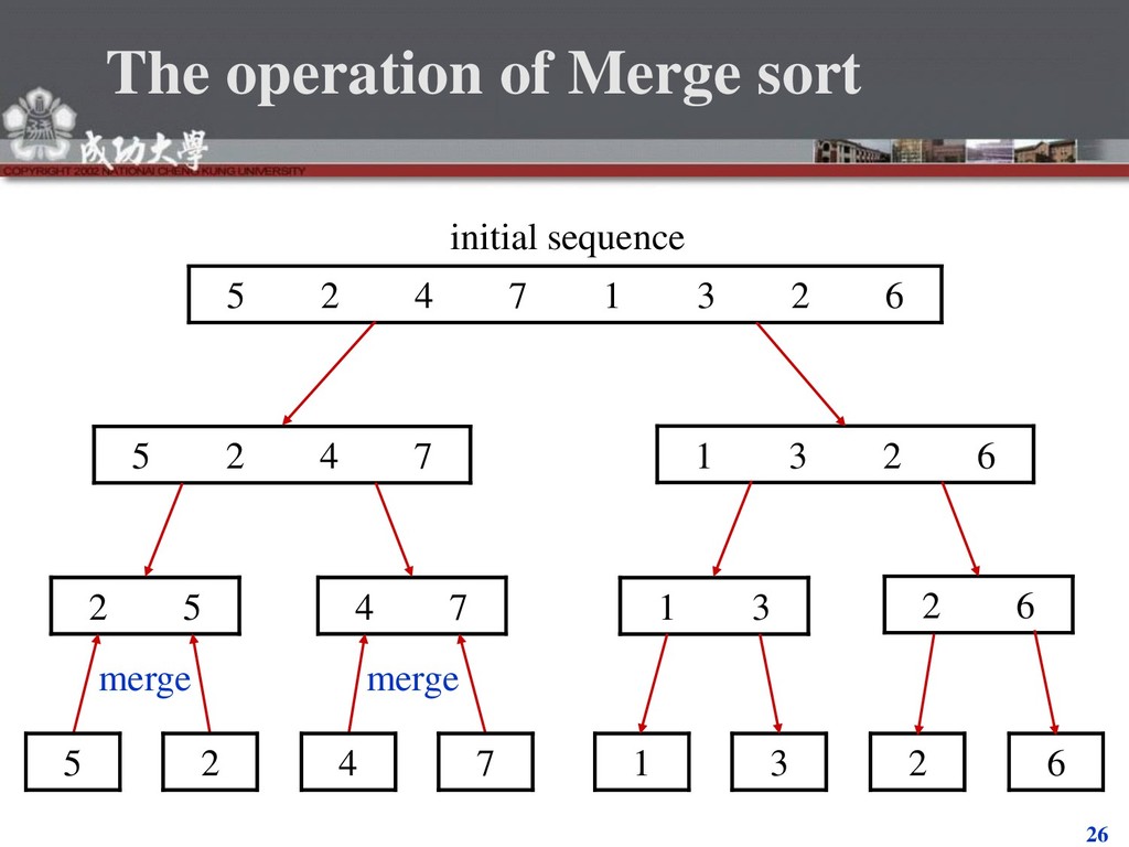
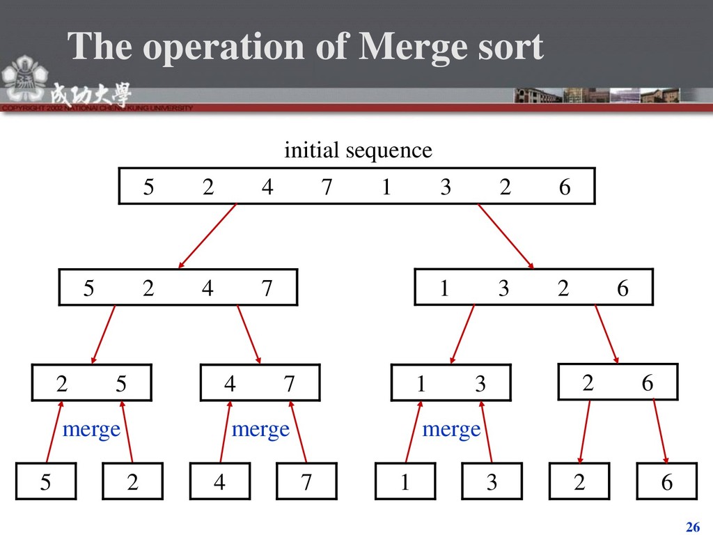
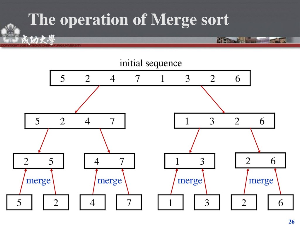
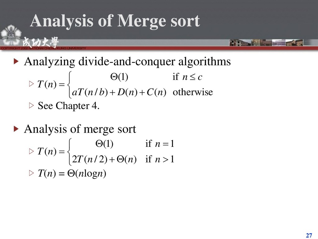
  12. 13 2.3 Designing algorithms There are many ways to design

    algorithms: Incremental approach: insertion sort Divide-and-conquer: merge sort recursive: divide conquer combine
  13. 14 Pseudocode Merge sort Merge(A, p, q, r) 1. n1

     q – p + 1 2. n2  r – q 3. create array L[1,…, n1 + 1] and R[1,…, n2 + 1] 4. for i  1 to n1 5. do L[i]  A[p + i – 1] 6. for j  1 to n2 7. do R[j]  A[q + j] 8. L[n1 + 1]   9. R[n2 + 1]  
  14. 15 Pseudocode 10. i  1 11. j  1

    12. for k  p to r 13. do if L[i]  R[j] 14. then A[k]  L[i] 15. i  i + 1 16. else A[k]  R[j] 17. j  j + 1
  15. 16 The operation of lines 10-17 8 9 10 11

    12 13 14 15 16 17 A … 2 4 5 7 1 2 3 6 … k 1 2 3 4 5 L 2 4 5 7  i 1 2 3 4 5 R 1 2 3 6  j (a)
  16. 17 The operation of lines 10-17 8 9 10 11

    12 13 14 15 16 17 A … 1 4 5 7 1 2 3 6 … k 1 2 3 4 5 L 2 4 5 7  i 1 2 3 4 5 R 1 2 3 6  j (b)
  17. 18 The operation of lines 10-17 8 9 10 11

    12 13 14 15 16 17 A … 1 2 5 7 1 2 3 6 … k 1 2 3 4 5 L 2 4 5 7  i 1 2 3 4 5 R 1 2 3 6  j (c)
  18. 19 The operation of lines 10-17 8 9 10 11

    12 13 14 15 16 17 A … 1 2 2 7 1 2 3 6 … k 1 2 3 4 5 L 2 4 5 7  i 1 2 3 4 5 R 1 2 3 6  j (d)
  19. 20 The operation of lines 10-17 8 9 10 11

    12 13 14 15 16 17 A … 1 2 2 3 1 2 3 6 … k 1 2 3 4 5 L 2 4 5 7  i 1 2 3 4 5 R 1 2 3 6  j (e)
  20. 21 The operation of lines 10-17 8 9 10 11

    12 13 14 15 16 17 A … 1 2 2 3 4 2 3 6 … k 1 2 3 4 5 L 2 4 5 7  i 1 2 3 4 5 R 1 2 3 6  j (f)
  21. 22 The operation of lines 10-17 8 9 10 11

    12 13 14 15 16 17 A … 1 2 2 3 4 5 3 6 … k 1 2 3 4 5 L 2 4 5 7  i 1 2 3 4 5 R 1 2 3 6  j (g)
  22. 23 The operation of lines 10-17 8 9 10 11

    12 13 14 15 16 17 A … 1 2 2 3 4 5 6 6 … k 1 2 3 4 5 L 2 4 5 7  i 1 2 3 4 5 R 1 2 3 6  j (h)
  23. 24 The operation of lines 10-17 8 9 10 11

    12 13 14 15 16 17 A … 1 2 2 3 4 5 6 7 … k 1 2 3 4 5 L 2 4 5 7  i 1 2 3 4 5 R 1 2 3 6  j (i)
  24. 25 Pseudocode MERGE-SORT(A, p, r) 1. if p < r

    2. then q  (p + r)/2 3. MERGE-SORT(A, p, q) 4. MERGE-SORT(A, q + 1, r) 5. MERGE(A, p, q, r)
  25. 26 The operation of Merge sort initial sequence 5 2

    4 7 1 3 2 6 5 2 4 7 1 3 2 6 5 2 4 7
  26. 26 The operation of Merge sort initial sequence 5 2

    4 7 1 3 2 6 5 2 4 7 1 3 2 6 5 2 2 6 4 7 1 3
  27. 26 The operation of Merge sort initial sequence 5 2

    4 7 1 3 2 6 5 2 4 7 1 3 2 6 5 2 2 6 4 7 1 3 5 2
  28. 26 The operation of Merge sort initial sequence 5 2

    4 7 1 3 2 6 5 2 4 7 1 3 2 6 5 2 2 6 4 7 1 3 5 2 4 7
  29. 26 The operation of Merge sort initial sequence 5 2

    4 7 1 3 2 6 5 2 4 7 1 3 2 6 5 2 2 6 4 7 1 3 5 2 4 7 1 3
  30. 26 The operation of Merge sort initial sequence 5 2

    4 7 1 3 2 6 5 2 4 7 1 3 2 6 5 2 2 6 4 7 1 3 5 2 4 7 1 3 2 6
  31. 26 The operation of Merge sort 2 5 initial sequence

    merge 5 2 4 7 1 3 2 6 5 2 4 7 1 3 2 6 2 6 4 7 1 3 5 2 4 7 1 3 2 6
  32. 26 The operation of Merge sort 2 5 4 7

    initial sequence merge merge 5 2 4 7 1 3 2 6 5 2 4 7 1 3 2 6 2 6 1 3 5 2 4 7 1 3 2 6
  33. 26 The operation of Merge sort 2 5 4 7

    1 3 initial sequence merge merge merge 5 2 4 7 1 3 2 6 5 2 4 7 1 3 2 6 2 6 5 2 4 7 1 3 2 6
  34. 26 The operation of Merge sort 2 5 2 6

    4 7 1 3 initial sequence merge merge merge merge 5 2 4 7 1 3 2 6 5 2 4 7 1 3 2 6 5 2 4 7 1 3 2 6
  35. 26 The operation of Merge sort 2 4 5 7

    2 5 2 6 4 7 1 3 initial sequence merge merge merge merge merge 5 2 4 7 1 3 2 6 1 3 2 6 5 2 4 7 1 3 2 6
  36. 26 The operation of Merge sort 2 4 5 7

    1 2 3 6 2 5 2 6 4 7 1 3 initial sequence merge merge merge merge merge merge 5 2 4 7 1 3 2 6 5 2 4 7 1 3 2 6
  37. 26 The operation of Merge sort 1 2 2 3

    4 5 6 7 2 4 5 7 1 2 3 6 2 5 2 6 4 7 1 3 sorted sequence merge merge merge merge merge merge merge 5 2 4 7 1 3 2 6
  38. 27 Analysis of Merge sort Analyzing divide-and-conquer algorithms See Chapter

    4. Analysis of merge sort T(n) = (nlogn) otherwise if ) ( ) ( ) / ( ) 1 ( ) ( c n n C n D b n aT n T         1 if 1 if ) ( ) 2 / ( 2 ) 1 ( ) (          n n n n T n T
  39. 28 Analysis of Merge sort where the constant c represents

    the time require to solve problem of size 1 as well as the time per array element of the divide and combine steps. 1 if 1 if ) 2 / ( 2 ) (        n n cn n T c n T
  40. 29 The construction of a recursion tree T(n) cn T(n/2)

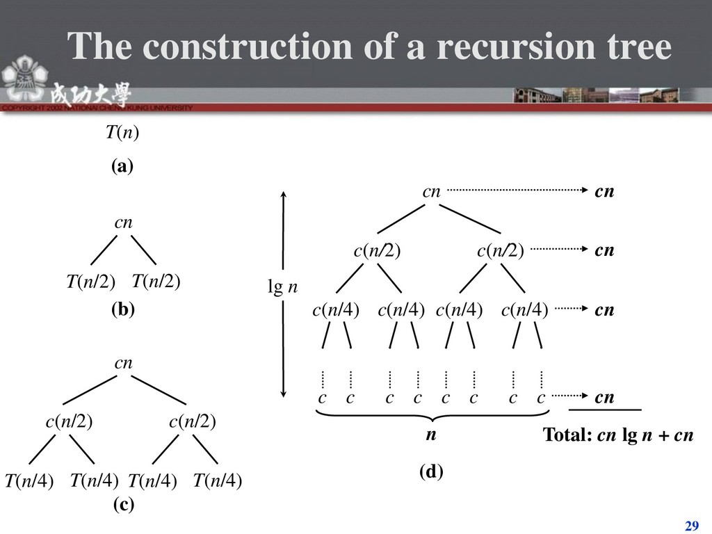
    T(n/2) c(n/2) T(n/4) T(n/4) c(n/2) T(n/4) T(n/4) cn (a) (b) (c) c(n/2) c(n/4) c(n/4) c(n/2) c(n/4) c(n/4) cn c c c c c c c c lg n n cn cn cn cn Total: cn lg n + cn (d)