Lyapunov Control for Flat Spin Recovery and Spin Inversion

I developed new control laws for stabilizing a tumbling spacecraft using reaction wheels. This presentation is from the 2016 AIAA Astrodynamics Specialist Conference.

Transcript

1. Zac  Manchester
   Harvard  Agile  Robotics  Lab
   (Formerly  Cornell  Space  Systems  Design  Studio)
   Lyapunov-­‐Based  Control  Laws  for
   Flat  Spin  Recovery  and  Spin  Inversion
   

   View Slide

2. 2
   Motivation
   

   View Slide

3. 3
   Problem:
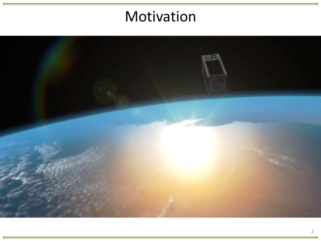
   • Achieve  spin  about  minor  axis  of  inertia  from  arbitrary  initial  conditions
   • Align  + face  of  the  spacecraft  with  the  angular  momentum  vector
   Constraints:
   • Limited  reaction  wheel  torque
   • Limited  angular  momentum  storage  in  reaction  wheels
   Motivation
   

   View Slide

4. 4
   Gyrostat  Dynamics:
   J = I 1
   ˙
   h = h ⇥ J ·(h ⇢)
   h = I·! + ⇢
   I· ˙
   ! + ! ⇥ (I·! + ⇢) + ˙
   ⇢ = ⌧
   Background
   

   View Slide

5. 0
   0.5
   1
   1.5
   2
   5
   Lyapunov Stability:
   ˙
   x
   =
   f
   (
   x
   )
   V
   (
   x
   ) 0
   ˙
   V
   (
   x
   ) = @V
   @x
   d
   x
   d
   t
    0
   f
   (
   x
   ⇤) = 0
   Background
   

   View Slide

6. 6
   Some  Candidates:
   VQ =
   1
   2
   hd
   ·J ·hd
   1
   2
   h·J ·h
   Lyapunov  Functions
   

   View Slide

7. 7
   Some  Candidates:
   VL = hd
   ·J ·hd hd
   ·J ·h
   Lyapunov  Functions
   

   View Slide

8. 8
   Periodic  Averaging:
   V 0
   L
   = hd
   ·J ·hd
   1
   T
   Z T
   0
   hd
   ·J ·h dt
   Lyapunov  Functions
   

   View Slide

9. 9
   Periodic  Averaging:
   V =
   3
   2
   hd
   ·J ·hd
   1
   T
   Z T
   0
   hd
   ·J ·h +
   1
   2
   h·J ·h dt
   Lyapunov  Functions
   

   View Slide

10. 10
    Discretization:
    hk = h(t0 + k t) ⇢k = ⇢(t0 + k t)
    xk =
    2
    6
    4
    hk
    .
    .
    .
    hk+N 1
    3
    7
    5 uk =
    2
    6
    4
    ⇢k
    .
    .
    .
    ⇢k+N 1
    3
    7
    5
    xd =
    2
    6
    4
    hd
    .
    .
    .
    hd
    3
    7
    5
    Calculating  ̇
    

    View Slide

11. 11
    Discretization:
    1
    T
    Z T
    0
    hd
    ·
    J
    · h +
    1
    2
    h ·
    J
    · h d
    t
    ⇡
    1
    N
    x
    |
    d
    ¯
    J xk +
    1
    2
    N
    x
    |
    k
    ¯
    J xk
    ¯
    J =
    2
    6
    6
    6
    4
    J 0 · · · 0
    0 J · · · 0
    .
    .
    .
    .
    .
    .
    ...
    .
    .
    .
    0 0 · · · J
    3
    7
    7
    7
    5
    Calculating  ̇
    

    View Slide

12. 12
    Periodic  System:
    A =
    2
    6
    6
    6
    6
    6
    6
    4
    0 13⇥3 0 · · · 0
    0 0 13⇥3
    .
    .
    . 0
    .
    .
    .
    .
    .
    .
    ...
    ...
    .
    .
    .
    0 0 · · · 0 13⇥3
    13⇥3 0 · · · 0 0
    3
    7
    7
    7
    7
    7
    7
    5
    Bk = t
    2
    6
    6
    6
    6
    4
    h⇥
    k
    J 0 · · · 0
    0 h⇥
    k+1
    J 0
    .
    .
    .
    .
    .
    .
    ...
    ... 0
    0 · · · 0 h⇥
    k+N 1
    J
    3
    7
    7
    7
    7
    5
    Calculating  ̇
    ˙
    h = h ⇥
    J
    ·(h ⇢) !
    xk+1 =
    Axk +
    Bkuk
    

    View Slide

13. 13
    Continuum  Limit:
    V
    =
    1
    N
    x
    |
    d
    ¯
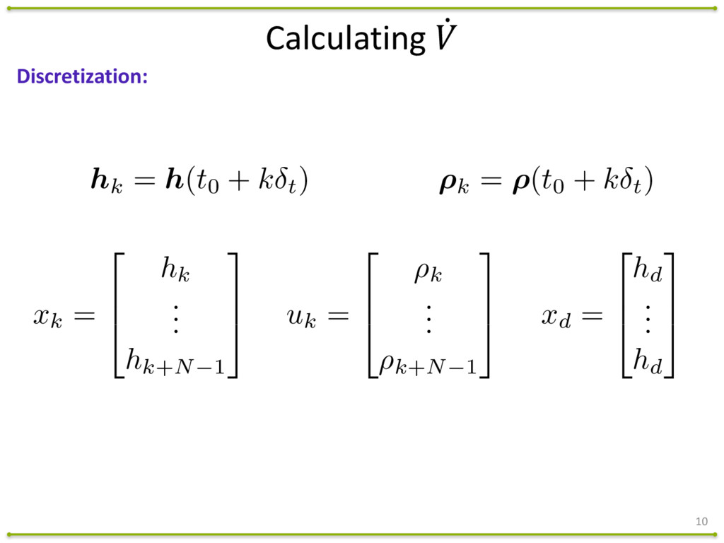
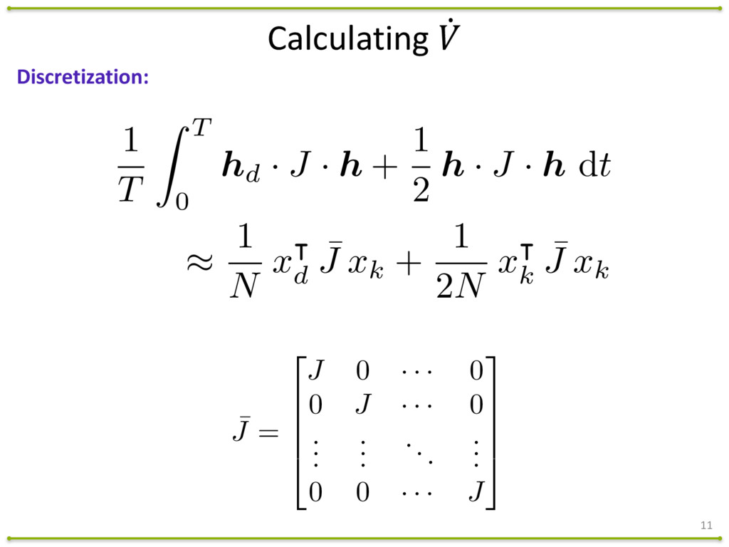
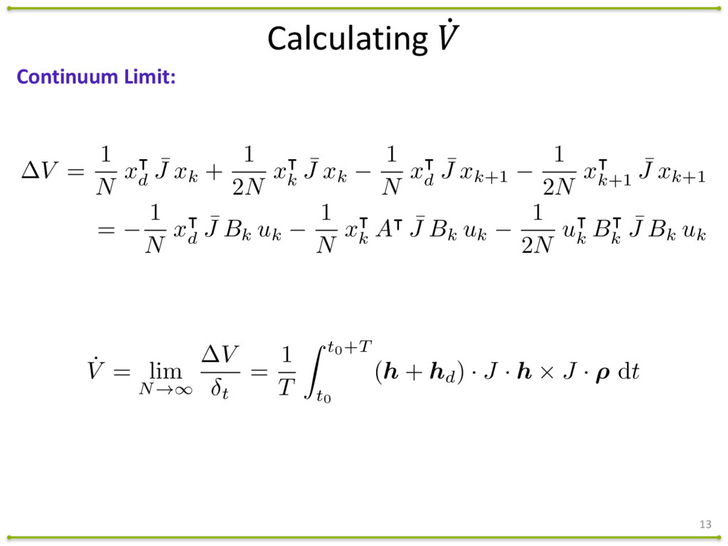
    J xk +
    1
    2
    N
    x
    |
    k
    ¯
    J xk
    1
    N
    x
    |
    d
    ¯
    J xk+1
    1
    2
    N
    x
    |
    k+1
    ¯
    J xk+1
    =
    1
    N
    x
    |
    d
    ¯
    J Bk uk
    1
    N
    x
    |
    k A
    | ¯
    J Bk uk
    1
    2
    N
    u
    |
    k B
    |
    k
    ¯
    J Bk uk
    ˙
    V = lim
    N!1
    V
    t
    =
    1
    T
    Z t0+T
    t0
    (h + hd) · J · h ⇥ J · ⇢ dt
    Calculating  ̇
    

    View Slide

14. 14
    Almost-­‐Global  Asymptotic  Stability:
    ˙
    V =
    1
    T
    Z T
    0
    (h + hd)·J ·h ⇥ J ·⇢ dt
    b(h)
    ⇢ ⇡ ⇢
    max
    sign(b)
    Control  Laws
    

    View Slide

15. 15
    Smooth  Control  Law:
    ⇢ = ⇢
    max
    tanh(↵b)
    x
    -5 0 5
    tanh(x)
    -1
    -0.8
    -0.6
    -0.4
    -0.2
    0
    0.2
    0.4
    0.6
    0.8
    1
    Control  Laws
    

    View Slide

16. 16
    Momentum  Vector  Trajectory:
    0.5
    0
    -0.5
    -1
    1
    0.5
    0
    -0.5
    0.5
    0
    -0.5
    1
    Flat-­‐Spin  Recovery
    

    View Slide

17. 0 2 4 6 8
    ;
    1
    -0.01
    0
    0.01
    0 2 4 6 8
    ;
    2
    -0.01
    0
    0.01
    Time (min)
    0 2 4 6 8
    ;
    3
    -0.01
    0
    0.01
    17
    Control  Inputs:
    Flat-­‐Spin  Recovery
    

    View Slide

18. 18
    Momentum  Vector  Trajectory:
    0.5
    0
    -0.5
    -0.5
    0
    0.5
    -1
    1
    0.8
    0.6
    0.4
    0.2
    0
    -0.2
    -0.4
    -0.6
    -0.8
    Spin  Inversion
    

    View Slide

19. 0 1 2 3 4 5 6
    ;
    1
    -0.01
    0
    0.01
    0 1 2 3 4 5 6
    ;
    2
    -0.01
    0
    0.01
    Time (min)
    0 1 2 3 4 5 6
    ;
    3
    -0.01
    0
    0.01
    19
    Control  Inputs:
    Spin  Inversion
    

    View Slide

20. 20
    zmanchester@seas.harvard.edu
    Questions?
    

    View Slide