Ph.D. Defense

Zac Manchester Centimeter-‐Scale Spacecraft: Design, Fabrication, and Deployment

Why? 1

”Space Transportation Costs: Trends in Price Per Pound to Orbit.”
Futron Corporation. Bethesda, MD. September 6, 2002. Expanding Access to Space

• Electronics are improving much faster Wikipedia Expanding Access to
Space

Shrink The Spacecraft! 4

Contributions 5 1. Design and fabrication of a complete spacecraft
on a printed circuit board 2. A CubeSat-‐based deployment system for centimeter-‐scale spacecraft 3. A Low-‐power, long-‐range communication system for centimeter-‐scale spacecraft 4. Feedback control laws capable of both flat-‐spin recovery and spin-‐axis inversion of spinning spacecraft 5. Variational integrators for spacecraft dynamics with quaternion state variables 6. An algorithm for recursive estimation of spacecraft inertia using semidefinite programming

Courses 6 Methods of Applied Math I (TAM 6100) Methods
of Applied Math II (TAM 6110) Numerical Analysis: Linear and Nonlinear Problems (CS 5223) Stochastic Systems: Estimation and Control (ECE 5555) Minor (Applied Math) Feedback Control Systems (MAE 4780) Intermediate Dynamics (TAM 5700) GPS: Theory and Design (MAE 4150) Spacecraft Dynamics (MAE 6060) Celestial Mechanics (TAM 6720) Computer Vision (ECE 5470) Theory of Linear Systems (MAE 5210) Differential Equations and Dynamical Systems (MATH 4200) Multivariable Control Theory (MAE 6780) Engineering Vibrations (MAE 5770) Model-‐Based Estimation (MAE 6760) Engineering

Publications To Date Manchester, Z. R., and Peck, M. A.,
“Quaternion Variational Integrators for Spacecraft Dynamics,” Journal of Guidance, Control, and Dynamics, 2015 (To Appear). Manchester, Z. R., Peck, M. A., and Filo, A.., “KickSat: A Crowd-‐Funded Mission To Demonstrate The World’s Smallest Spacecraft,” AIAA/USU Conference on Small Satellites, Logan, Utah, August 12-‐16, 2013. Manchester, Z. R., and Peck, M. A., “Stochastic Space Exploration with Microscale Spacecraft,” AIAA Guidance, Navigation, and Control Conference, Portland, OR, August 8-‐11, 2011. Atchison, J. A., Manchester, Z. R., and Peck, M. A., "Microscale Atmospheric Reentry Sensors," 7th International Planetary Probe Workshop, Barcelona, Spain, June 14-‐18, 2010. 7

Publications To Be Submitted (In Thesis): Manchester, Z. R., and
Peck, M. A., “Recursive Spacecraft Inertia Estimation with Semidefinite Programming,” Journal of Guidance, Control, and Dynamics. Manchester, Z. R., and Peck, M. A., “Lyapunov-‐Based Control for Flat-‐Spin Recovery and Spin Inversion of Spin-‐Stabilized Spacecraft,” Journal of Guidance, Control, and Dynamics. Manchester, Z. R., and Peck, M. A., “The Sprite: A Centimeter-‐Scale Spacecraft,” Journal of Spacecraft and Rockets. 8

Centimeter-‐Scale Spacecraft 9

10 Literature Survey: Janson, S. W., “Mass-‐Producible Silicon Spacecraft
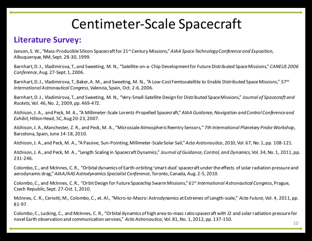
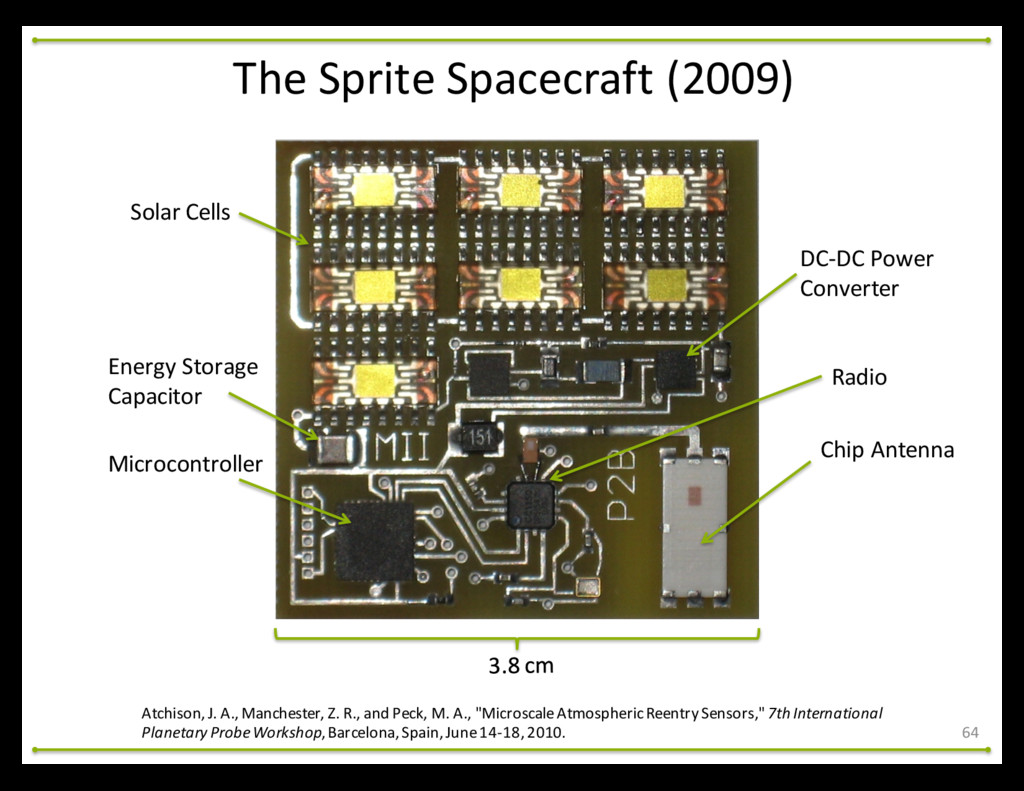
for 21st Century Missions,” AIAA Space Technology Conference and Exposition, Albuquerque, NM, Sept. 28-‐30, 1999. Barnhart, D. J., Vladimirova, T., and Sweeting, M. N., “Satellite-‐on-‐a-‐ Chip Development for Future Distributed Space Missions,” CANEUS 2006 Conference, Aug. 27-‐Sept. 1, 2006. Barnhart, D. J., Vladimirova, T., Baker, A. M., and Sweeting, M. N., “A Low-‐Cost Femtosatellite to Enable Distributed Space Missions,” 57th International Astronautical Congress, Valencia, Spain, Oct. 2-‐6, 2006. Barnhart, D. J., Vladimirova, T., and Sweeting, M. N., “Very-‐Small-‐Satellite Design for Distributed Space Missions,” Journal of Spacecraft and Rockets, Vol. 46, No. 2, 2009, pp. 469-‐472. Atchison, J. A., and Peck, M. A., “A Millimeter-‐Scale Lorentz-‐Propelled Spacecraft,” AIAA Guidance, Navigation and Control Conference and Exhibit, Hilton Head, SC, Aug 20-‐23, 2007. Atchison, J. A., Manchester, Z. R., and Peck, M. A., "MicroscaleAtmospheric Reentry Sensors," 7th International Planetary Probe Workshop, Barcelona, Spain, June 14-‐18, 2010. Atchison, J. A., and Peck, M. A., “A Passive, Sun-‐Pointing, Millimeter-‐Scale Solar Sail,” Acta Astronautica, 2010, Vol. 67, No. 1, pp. 108-‐121. Atchison, J. A., and Peck, M. A., “Length Scaling in Spacecraft Dynamics,” Journal of Guidance, Control, and Dynamics, Vol. 34, No. 1, 2011, pp. 231-‐246. Colombo, C., and McInnes, C. R., “Orbital dynamics of Earth-‐orbiting ‘smart-‐dust’ spacecraft under the effects of solar radiation pressure and aerodynamic drag,” AIAA/AAS Astrodynamics Specialist Conference, Toronto, Canada, Aug. 2-‐5, 2010. Colombo, C., and McInnes, C. R., “Orbit Design for Future Spacechip Swarm Missions,” 61st International Astronautical Congress, Prague, Czech Republic, Sept. 27-‐Oct. 1, 2010. McInnes, C. R., Ceriotti, M., Colombo, C., et. Al., “Micro-‐to-‐Macro: Astrodynamicsat Extremes of Length-‐scale,” Acta Futura, Vol. 4, 2011, pp. 81-‐97. Colombo, C., Lucking, C., and McInnes, C. R., “Orbital dynamics of high area-‐to-‐mass ratio spacecraft with J2 and solar radiation pressure for novel Earth observation and communication services,” Acta Astronautica, Vol. 81, No. 1, 2012, pp. 137-‐150. Centimeter-‐Scale Spacecraft

Centimeter-‐Scale Spacecraft Returned To Earth (5/18/2014): 14

Video Courtesy Ben Bishop 15 KickSat Mission Concept: Centimeter-‐Scale
Spacecraft

16 Deployment Testing: Centimeter-‐Scale Spacecraft

Centimeter-‐Scale Spacecraft 17 Launch (4/18/2014):

18 Problem: How can we communicate with hundreds of small
spacecraft simultaneously? Constraints: • Transmitter power is limited (10 mW) • Spacecraft antenna must have low gain due to lack of pointing capability • Licensing (only one frequency allocation for the entire “swarm”) Communication

19 Communication Clean Signal:

20 Communication Received Signal:

21 Communication Clean Signal:

22 Communication Received Signal:

23 Communication Matched Filter: Template: 1 1 1 1 1
0 0 1 1 0 1 0 1 1 1 0 0 1 1 1 0 0 1 1 0 0 1 0 1 1 1 0 0 0 0 1 0 1 1 0 0 0 0 0 1 0 0 1 0 1 1 0 1 1 1 1 1 0 0 1 1 0 1 0 1 20 30 40

Communication 24 PRN Sequence: • Long deterministically-‐generated sequences of
bits • Look like noise (approximate δ-‐function autocorrelation) Gold Codes: • Commonly used code family (e.g. in GPS) • Easily generated by a linear feedback shift register (or a few lines of code) • Low bounded cross-‐correlation among members of the family • 511 bit codes used for KickSat mission

25 Communication Received Signal After Matched Filter:

26 Communication Reciever:

27 Communication Testing:

Flat-‐Spin Recovery 28 Problem: How do we ensure KickSat’s angular
momentum vector is aligned with its +z axis? Constraints: • Very limited reaction wheel torque (3.8 mNm) • Very limited angular momentum storage in reaction wheels (.5 mNms)

29 Literature Survey: Bracewell, R. N., and Garriott, O.
K., “Rotation of Artificial Earth Satellites,” Nature, Vol. 182, Sept., 1958, pp. 760-‐762. Barba, P. M., Furumoto, N., and Leliakov, I. P., “Techniques for Flat-‐Spin Recovery of Spinning Satellites,” AIAA Guidance and Control Conference, Key Biscayne, Florida, Aug. 20-‐22, 1973. Gebman, J. R., and Mingori, D. L., “Perturbation Solution for the Flat Spin Recovery of a Dual-‐Spin Spacecraft,” AIAA Journal, Vol. 14, No. 7, July, 1976. Cronin, D. L., "Flat Spin Recovery of a Rigid Asymmetric Spacecraft", Journal of Guidance, Control, and Dynamics, Vol. 1, No. 4, 1978, pp. 281-‐282. Beachley, N. H. and Uicker, J. J., “Wobble-‐Spin Technique for Spacecraft Inversion and Earth Photography,” Journal of Spacecraft and Rockets, Vol. 6, No. 3, March 1969, pp. 245-‐248. Beachley, N. H., “Inversion of Spin-‐Stabilized Spacecraft by Mass Translation – Some Practical Aspects,” Journal of Spacecraft and Rockets, Vol. 8, No. 10, Oct. 1971, pp. 1078-‐1080 Rahn, C. D., and Barba, P. M., “Reorientation Maneuver for Spinning Spacecraft,” Journal of Guidance, Control, and Dynamics, Vol. 14, No. 4, July 1991, pp. 724-‐728. Rand, R. H., and Hall, C. D., “Spinup Dynamics of Axial Dual-‐Spin Spacecraft,” Journal of Guidance, Control, and Dynamics, Vol. 17, No. 1, 1994, pp. 30-‐37. Chaturvedi, N. A., Bernstein, D. S., Ahmed, J., Bacconi, F., and McClamroch, N. H., “Globally Convergent Adaptive Tracking of Angular Velocity and Inertia Identification for a 3-‐DOF Rigid Body,” IEEE Transactions on Control Systems Technology, Vol. 14, No. 5, Sept., 2006. Lawrence, D. A., and Holden, T. E., “Essentially Globally Asymptotically Stable Nutation Control Using a Single Reaction Wheel,” Journal of Guidance, Control, and Dynamics, Vol. 30, No. 6, Nov.-‐Dec., 2007. Myung, H. S., and Bang, H., “Predictive Nutation and Spin Inversion Control of Spin-‐Stabilized Spacecraft,” Journal of Spacecraft and Rockets, Vol. 47, No. 6, Nov.-‐Dec., 2010. Flat-‐Spin Recovery

Flat-‐Spin Recovery 30 Gyrostat Dynamics: J = I 1 ˙
h = h ⇥ J ·(h ⇢) h = I·! + ⇢ I· ˙ ! + ! ⇥ (I·! + ⇢) + ˙ ⇢ = ⌧

0 0.5 1 1.5 2 Flat-‐Spin Recovery 31 Lyapunov Stability:
˙ x = f ( x ) V ( x ) 0 ˙ V ( x ) = @V @x d x d t  0 f ( x ⇤) = 0

Flat-‐Spin Recovery 32 Candidate Lyapunov Functions: VQ = 1 2
hd ·J ·hd 1 2 h·J ·h VL = hd ·J ·hd hd ·J ·h

Flat-‐Spin Recovery 33 Periodic Averaging: V 0 L = hd
·J ·hd 1 T Z T 0 hd ·J ·h dt

Flat-‐Spin Recovery 34 Periodic Averaging: V = 3 2 hd
·J ·hd 1 T Z T 0 hd ·J ·h + 1 2 h·J ·h dt

Flat-‐Spin Recovery 35 Control Law: ˙ V = 1 T
Z T 0 (h + hd)·J ·h ⇥ J ·⇢ dt b(h) ⇢ ⇡ ⇢ max sign(b)

Flat-‐Spin Recovery 36 Control Law: ⇢ = ⇢ max tanh(↵b)
x -5 0 5 tanh(x) -1 -0.8 -0.6 -0.4 -0.2 0 0.2 0.4 0.6 0.8 1

Flat-‐Spin Recovery 37 Flat-‐Spin Recovery Simulation: 0.5 0 -0.5 -1
1 0.5 0 -0.5 0.5 0 -0.5 1

Flat-‐Spin Recovery 38 Spin-‐Inversion Simulation: 0.5 0 -0.5 -0.5 0
0.5 -1 1 0.8 0.6 0.4 0.2 0 -0.2 -0.4 -0.6 -0.8

Discrete Variational Mechanics 39 Motivation: • Variational integrators have many
advantages over e.g. Runge-‐Kutta schemes • Well suited for use in estimation and control applications • Theory is based on Lagrangian and/or Hamiltonian Mechanics ⇒ Need a Lagrangian formulation of attitude dynamics! L = T V = 1 2 !·I·! S = Z tf t0 1 2 !·I·! dt = ?

40 Literature Survey: Moser, J., and Veselov, A. P.,
“Discrete Versions of Some Classical Integrable Systems and Factorizations of Matrix Polynomials,” Communications in Mathematical Physics, Vol. 139, 1991, pp. 217-‐243. McLachlan, R. I., “Explicit Lie-‐Poisson Integration and the Euler Equations,” Physical Review Letters, Vol. 71, 1993, pp. 3043-‐ 3046. Reich, S. “Numerical Integration of the Generalized Euler Equations,” Technical Report 93-‐20, Department of Computer Science, University of British Columbia, 1993. Marsden, J. E., and West, M., “Discrete mechanics and variational integrators,” Acta Numerica, Vol. 10, 2001, pp. 357-‐514. Lee, T., Leok, M., and McClamroch, N. H., “A Lie Group Variational Integrator for the Attitude Dynamics of a Rigid Body with Applications to the 3D Pendulum,” IEEE Conference on Control Applications, Toronto, Canada, Aug. 28-‐31, 2005. Hussein, I. I., Leok, M., Sanyal, A. K., and Block, A. M., “A Discrete Variational Integrator for Optimal Control Problems on SO(3),” IEEE Conference on Decision & Control, San Diego, CA, Dec. 13015, 2006. Lee, T., Leok, M., and McClamroch, N. H., “Lie group variational integrators for the full body problem,” Computer methods in applied mechanics and engineering, Vol. 196, 2007, pp. 2907-‐2924. Krysl, P., “Direct time integration of rigid body motion with discrete-‐impulse midpoint approximation: Explicit Newmark algorithms,” Communications in Numerical Methods in Engineering, Vol. 22, 2006, pp. 441-‐451. Saccon, A., “Midpoint rule for variational integrators on Lie groups,” International Journal for Numerical Methods in Engineering, Vol. 78, 2009, pp. 1345-‐1364. Discrete Variational Mechanics

41 Quaternions: Discrete Variational Mechanics r ✓ q = 2
6 6 4 q1 q2 q3 q4 3 7 7 5 = 2 6 6 4 qv qs 3 7 7 5 = 2 6 6 4 r sin( ✓/ 2) cos( ✓/ 2) 3 7 7 5

42 Hamilton’s Principle: Discrete Variational Mechanics =) I· ˙ !
+ ! ⇥ (I·!) = 0 S = d d✏ ✏=0 Z tf t0 1 2 ✏ ˆ !· ˆ I·✏ ˆ ! dt = 0

43 Discrete Action Sum: Discrete Variational Mechanics S = Z
tf t0 1 2 ˆ !· ˆ I·ˆ ! dt = N X k=0 Z tk+1 tk 1 2 ˆ !· ˆ I·ˆ ! dt S ⇡ Sd = N X k=0 2 ⌧ fk · ˆ I · fk

44 Discrete Hamilton’s Principle: Discrete Variational Mechanics Sd = d
d✏ ✏=0 N X k=0 1 2 ✏fk · ˆ I·✏fk = 0 =) p 1 k · k I· k k ⇥ I· k = p 1 k+1 · k+1 I· k+1 + k+1 ⇥ I· k+1 fk = 2 6 6 4 k p 1 k · k 3 7 7 5

45 Free Rigid Body Simulation: Discrete Variational Mechanics 0 2
4 6 8 10 0 5 10 15 20 25 Time (min) Error (%) Variational Midpoint ODE45 Momentum Error (%)

46 Free Rigid Body Simulation: Discrete Variational Mechanics 0 2
4 6 8 10 0 2 4 6 8 Time (min) Error (%) Variational Midpoint ODE45 Energy Error (%)

47 Kalman Filtering: Discrete Variational Mechanics 10−1 100 101 102
0 10 20 30 40 50 Sample Rate (Hz) RMS Error (deg) Standard MEKF Variational MEKF

Inertia Estimation 48 Problem: • Inertia knowledge is needed for
control of KickSat’s spin axis • Accurate ground-‐based inertia measurements require expensive specialized equipment

49 Literature Survey: Bergmann, E. V., Walker, B. K., and
Levy, D. R., “Mass Property Estimation for Control of Asymmetrical Satellites,” Journal of Guidance, Control, and Dynamics, Vol. 10, No. 5, 1987, pp. 483-‐491. Tanygin, S. and Williams, T., “Mass Property Estimation Using Coasting Maneuvers,” Journal of Guidance, Control, and Dynamics, Vol. 20, No. 4, 1997, pp. 625-‐632. Ahmed, J., Coppola, V. T., and Bernstein, D. S., “Adaptive Asymptotic Tracking of Spacecraft Attitude Motion with Inertia Matrix Identification,” Journal of Guidance, Control, and Dynamics, Vol. 21, No. 5, 1998, pp. 684-‐691. Psiaki, M. L., “Estimation of a Spacecraft’s Attitude Dynamics Parameters by Using Flight Data,” Journal of Guidance, Control, and Dynamics, Vol. 28, No. 4, 2005, pp. 594-‐603. Peck, M. A., “Uncertainty Models for Physically Realizable Inertia Dyadics,” Journal of the AstronauticalSciences, Vol. 54, No. 1, 2006, pp. 1-‐16. Norman, M. C., Peck, M. A., and O’Shaghnessy, D. J., “In-‐orbit Estimation of Inertia and Momentum-‐Actuator Alignment Parameters,” Journal of Guidance, Control, and Dynamics, Vol. 34, No. 6, 2011, pp. 1798-‐1814. Keim, J. A., Acikmese, A., and Shields, J. F., “Spacecraft Inertia Estimation via Constrained Least Squares,” Proceedings of the IEEE Aerospace Conference, 2006. Inertia Estimation

50 A Least-‐Squares Problem: Inertia Estimation I· ˙ ! +
! ⇥ (I·! + ⇢) + ˙ ⇢ = ⌧ H(!, ˙ !)i = y(!, ⇢, ˙ ⇢, ⌧) i = ⇥ I11 I22 I33 I12 I13 I23 ⇤|

51 A Least-‐Squares Problem: Inertia Estimation q 1 k+1 ·
k+1 (I· k+1 + h 2 ⇢k+1 ) + k+1 ⇥ (I· k+1 + h 2 ⇢k+1 ) + h2 2 ⌧k+1 = p 1 k · k (I· k + h 2 ⇢k ) k ⇥ (I· k + h 2 ⇢k ) H( k , k+1 )i = y( k , k+1 , ⇢k , ⇢k+1 , ⌧k+1)

52 A Least-‐Squares Problem: Inertia Estimation minimize i kHi yk2
2 subject to ( I > 0 Ijj + Ikk Ill 0

53 Semidefinite Programming: Inertia Estimation minimize x c | x
subject to F0 + n X i =1 xiFi 0 Fi 2 Sn F 0 =) v| Fv 0 8 v 2 Rn

54 Schur Complement: Inertia Estimation =) ( C > 0
A BC 1B| 0  A B B| C 0

55 Semidefinite Program: Inertia Estimation minimize ⇥ · · ·
0 · · · 1 ⇤  i s subject to 8 > > > > > > > > < > > > > > > > > :  s ( Hi y ) | ( Hi y ) 1 0 I > 0 I11 + I22 I33 0 I11 + I33 I22 0 I22 + I33 I11 0

56 Simulation: Inertia Estimation 0 10 20 30 40 50
60 ! 1 -0.2 0 0.2 0 10 20 30 40 50 60 ! 2 -0.2 -0.1 0 0.1 Time (s) 0 10 20 30 40 50 60 ! 3 0.76 0.77 0.78 0.79 0 10 20 30 40 50 60 ; 1 -0.05 0 0.05 0 10 20 30 40 50 60 ; 2 -0.05 0 0.05 Time (s) 0 10 20 30 40 50 60 ; 3 -0.05 0 0.05

57 Simulation: Inertia Estimation 0 10 20 30 40 50
60 J 11 10-8 10-6 10-4 10-2 100 Momentum Based SDP Based 0 10 20 30 40 50 60 J 22 10-8 10-6 10-4 10-2 100 Time (s) 0 10 20 30 40 50 60 J 33 10-8 10-6 10-4 10-2 100 0 10 20 30 40 50 60 J 12 10-8 10-6 10-4 10-2 100 0 10 20 30 40 50 60 J 13 10-8 10-6 10-4 10-2 100 Time (s) 0 10 20 30 40 50 60 J 23 10-8 10-6 10-4 10-2 100

Acknowledgements Becky Manchester Justin Atchison Phillipe Tosi Matt Reyes Andy
Filo Pete Worden John Hines Harry Partridge Elwood Agasid Jasper Wolfe Cedric Priscal Oriol Tintore Gazulla Alberto Guillen Salas Ken Oyadomari Watson Attai Justin Manchester Scott Higginbotham Ryan Nugent

Questions? 59

Backup Slides

• Launch costs are not dropping very quickly: 1995: •
Average: $36,200/kg (Futron*, inflation adjusted) 2015: • Atlas V: $35,000/kg (ULA Website) • Falcon 9: $12,619/kg (SpaceX Website) ”Space Transportation Costs: Trends in Price Per Pound to Orbit.” Futron Corporation. Bethesda, MD. September 6, 2002. * Expanding Access to Space

• Weather/Climate • Ionospheric Physics C-‐REX Mission, NASA 62 Applications

• Planetary Exploration • Gravimetry Draper Labs Applications 63

Solar Cells Microcontroller Radio Chip Antenna Energy Storage Capacitor DC-‐DC
Power Converter The Sprite Spacecraft (2009) Atchison, J. A., Manchester, Z. R., and Peck, M. A., "MicroscaleAtmospheric Reentry Sensors," 7th International Planetary Probe Workshop, Barcelona, Spain, June 14-‐18, 2010. 64

Bifilar Pendulum 65 I ¨ ✓ + mgr2 sin( ✓
) p L2 2 r2 (1 cos( ✓ )) ⇡ I ¨ ✓ + mgr2 L ✓ = 0 !2 = mgr2 IL =) I = mgr2 !2L I, m L 2r L s h s r r θ h = p L2 2 r2 (1 cos( ✓ )) s2 = 2 r2 (1 cos( ✓ )) L = 1 2 I ˙ ✓2 + mg p L2 2 r2 (1 cos( ✓ ))

66 KickSat

That’s Us!

Centimeter-‐Scale Spacecraft Mission Operations:

72 Vibration Testing: Centimeter-‐Scale Spacecraft

73 Thermal Vacuum Testing: Centimeter-‐Scale Spacecraft

74 Thermal Vacuum Testing: Centimeter-‐Scale Spacecraft

75 Mass Properties Measurement: Centimeter-‐Scale Spacecraft

76 Centimeter-‐Scale Spacecraft Integration (12/3/2013):

ChipSat Spread 77

ChipSat Spread 78

Orbital Lifetime 79 0 5 10 15 20 25 50
100 150 200 250 300 350 Altitude vs. Time With No Attitude Control Time (days) Altitude (km)

80 Literature Survey: Ageev, D. V., “Bases of the Theory
of Linear Selection. Code Demultiplexing,” Proceedings of the Leningrad Experimental Institute of Communication, Vol. 3, No. 35, 1935. Shannon, C. E., Weaver, W., The Mathematical Theory of Communication, University of Illinois Press, 1949. Gold, R., “Optimal binary sequences for spread spectrum multiplexing,” IEEE Transactions on Information Theory, Vol. 13, No. 4, Oct. 1967, pp. 619-‐621. Welch, L.R., “Lower Bounds on the Maximum Cross Correlation of Signals,” IEEE Transactions on Information Theory, Vol. 20, No. 3, May 1974, pp. 397–399. Gilhousen, K. S., Jacobs, I. M., Padovani, R., et. Al., “On the Capacity of a Cellular CDMA System,” IEEE Transactions on Vehicular Technology, Vol. 40, No. 2, May, 1991. Kohno, R., Meidan, R., and Milstein, L. B., “Spread Spectrum Access Methods for Wireless Communications,” IEEE Communications Magazine, Jan. 1995. Viterbi, A. J., CDMA: Principles of Spread Spectrum Communication, Addison-‐Wesley, 1995. Misra, P., Enge, P., Global Positioning System: Signals, Measurements, and Performance, Ganga-‐Jamuna Press, Lincoln, MA, 2001. Blossom, E., “GNU Radio: Tools for Exploring the Radio Frequency Spectrum,” Linux Journal, URL: http://www.linuxjournal.com/article/7319 [cited 11 February 2013]. Communication

81 Communication Shannon-‐Hartley Theorem: • Channel is assumed to be
corrupted with Gaussian white noise • B = Bandwidth • S = Signal Power • N = Noise Power • C = Channel Capacity (bits/sec) C = B Log2 ✓ 1 + S N ◆

Communication 82 CDMA: • Assign each user a PRN code
• For every data bit, transmit a PRN code • Receiver separates signals using matched filters • All users can transmit simultaneously without coordination Caveats: • Must handle frequency offset between transmitter and receiver (e.g. Doppler) • Inter-‐user interference leads to upper bound on number of simultaneous users //Transmit data byte byte & BIT7 ? transmitRaw(prn1) : transmitRaw(prn0); byte & BIT6 ? transmitRaw(prn1) : transmitRaw(prn0); byte & BIT5 ? transmitRaw(prn1) : transmitRaw(prn0); byte & BIT4 ? transmitRaw(prn1) : transmitRaw(prn0); byte & BIT3 ? transmitRaw(prn1) : transmitRaw(prn0); byte & BIT2 ? transmitRaw(prn1) : transmitRaw(prn0); byte & BIT1 ? transmitRaw(prn1) : transmitRaw(prn0); byte & BIT0 ? transmitRaw(prn1) : transmitRaw(prn0);

Communication 83 Number of Simultaneous Users: P on = n!
Dk(1 D)( n k ) k! (n k)!

Communication 84 Forward Error Correction: • We don’t have a
“back channel” to request re-‐transmission if a byte is corrupted • Add redundant information to the message to help detect and correct errors Linear Block Codes: • Simplest forward error correction technique • Multiply message vector by code’s generator matrix to create code vector ⇥ · · · · · · c · · · · · · ⇤ 1⇥16 = ⇥ · · · m · · · ⇤ 1⇥8 2 6 6 6 6 6 6 6 6 6 6 4 1 0 0 1 1 1 1 0 1 0 0 0 0 0 0 0 0 1 0 0 1 1 1 0 0 1 0 0 0 0 0 0 1 1 0 0 1 1 0 1 0 0 1 0 0 0 0 0 0 1 1 0 0 1 1 1 0 0 0 1 0 0 0 0 0 0 1 1 0 0 1 1 0 0 0 0 1 0 0 0 1 1 1 1 0 0 1 0 0 0 0 0 0 1 0 0 0 1 1 1 1 0 0 0 0 0 0 0 0 0 1 0 1 1 0 1 0 1 1 1 0 0 0 0 0 0 0 1 3 7 7 7 7 7 7 7 7 7 7 5 16⇥8 G z }| {

Communication 85 Hamming Distance: • Minimum 1-‐norm distance between code
vectors • Measure of code’s error correcting power Maximum Likelihood Soft Decoder: • Take dot product of received code vector against all possible code vectors in Rn • Output is message vector corresponding to largest dot product • Scales poorly as message length increases c1 c2 c3 r

86 Communication GNURadio:

Flat-‐Spin Recovery 87 Lyapunov Stability: V = 1 2m ˙
x 2 + 1 2kx 2  ˙ x ¨ x =  0 1 k/m c/m  x ˙ x ˙ V = c ˙ x 2 m ¨ x + c ˙ x + kx = 0

Flat-‐Spin Recovery 88 Control Law: hk = h(t0 + k
t) ⇢k = ⇢(t0 + k t) xk = 2 6 4 hk . . . hk+N 1 3 7 5 uk = 2 6 4 ⇢k . . . ⇢k+N 1 3 7 5 1 T Z T 0 hd · J · h + 1 2 h · J · h d t ⇡ 1 N x | d ¯ J xk + 1 2 N x | k ¯ J xk xd = 2 6 4 hd . . . hd 3 7 5 ¯ J = 2 6 6 6 4 J 0 · · · 0 0 J · · · 0 . . . . . . ... . . . 0 0 · · · J 3 7 7 7 5

Flat-‐Spin Recovery 89 Control Law: xk+1 = Axk + Bkuk
A = 2 6 6 6 6 6 6 4 0 13⇥3 0 · · · 0 0 0 13⇥3 . . . 0 . . . . . . ... ... . . . 0 0 · · · 0 13⇥3 13⇥3 0 · · · 0 0 3 7 7 7 7 7 7 5 Bk = t 2 6 6 6 6 4 h⇥ k J 0 · · · 0 0 h⇥ k+1 J 0 . . . . . . ... ... 0 0 · · · 0 h⇥ k+N 1 J 3 7 7 7 7 5

0 2 4 6 8 _ ;1 -0.1 0 0.1
0 2 4 6 8 _ ;2 -0.1 0 0.1 Time (min) 0 2 4 6 8 _ ;3 -0.02 0 0.02 0 2 4 6 8 ; 1 -0.01 0 0.01 0 2 4 6 8 ; 2 -0.01 0 0.01 Time (min) 0 2 4 6 8 ; 3 -0.01 0 0.01 Flat-‐Spin Recovery 91 Flat-‐Spin Recovery Simulation:

0 1 2 3 4 5 6 _ ;1 -0.1
0 0.1 0 1 2 3 4 5 6 _ ;2 -0.1 0 0.1 Time (min) 0 1 2 3 4 5 6 _ ;3 -0.02 0 0.02 0 1 2 3 4 5 6 ; 1 -0.01 0 0.01 0 1 2 3 4 5 6 ; 2 -0.01 0 0.01 Time (min) 0 1 2 3 4 5 6 ; 3 -0.01 0 0.01 Flat-‐Spin Recovery 92 Spin-‐Inversion Simulation:

93 Quaternions: Discrete Variational Mechanics pq = 2 6 6
4 psqv + qspv + pv ⇥ qv psqs pv · qv 3 7 7 5 q† = 2 6 6 4 qv qs 3 7 7 5 q = 2 6 6 4 r sin( ✓/ 2) cos( ✓/ 2) 3 7 7 5 v0 = qvq† ˆ v = 2 6 6 4 v 0 3 7 7 5

94 Quaternions: Discrete Variational Mechanics ˆ ! = 2q† ˙
q = 2 6 6 4 ! 0 3 7 7 5 q† = 2 6 6 4 qv qs 3 7 7 5 ˆ I = 2 6 6 4 I11 I12 I13 0 I21 I22 I23 0 I31 I32 I33 0 0 0 0 0 3 7 7 5 L = 1 2 ˆ !· ˆ I·ˆ !

95 Quaternion Exponential: Discrete Variational Mechanics eq = eqs 2
6 6 4 qv kqv k sin( kqv k ) cos( kqv k ) 3 7 7 5 = eˆ r✓/2

96 Hamilton’s Principle: Discrete Variational Mechanics ˆ ! = 2q†
˙ q =) ✏ ˆ ! = e ✏ˆ ⌘ ˆ !e✏ˆ ⌘ + 2✏ ˙ ˆ ⌘ =) I· ˙ ! + ! ⇥ (I·!) = 0 S = d d✏ ✏=0 Z tf t0 1 2 ✏ ˆ !· ˆ I·✏ ˆ ! dt ✏ ˙ q = ˙ qe✏ˆ ⌘ + ✏q✏ ˙ ˆ ⌘ ✏q = qe✏ˆ ⌘

97 Simulation with Kane Damper: Discrete Variational Mechanics 10−1 100
101 102 0 10 20 30 40 50 60 Damping Constant Running Time (sec) ODE45 Variational ! !d

98 Simulation with Kane Damper: Discrete Variational Mechanics ! !d
0 100 200 300 1.22 1.225 1.23 1.235 1.24 1.245 Time (sec) Energy ODE45 Variational

99 Simulation with Kane Damper: Discrete Variational Mechanics 0 100
200 300 1.22 1.23 1.24 1.25 1.26 1.27 1.28 Time (sec) Energy ODE15s Variational ! !d

Ph.D. Defense

Ph.D. Defense

More Decks by Zac Manchester

Other Decks in Research

Featured

Transcript