Katz, Michael Wilde Ketan Maheshwari, Ian Foster Scott Callaghan, Phillip Maechling *Department of Computer Science University of Chicago 2011 July 20 1 / 32
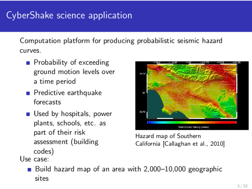
curves. Probability of exceeding ground motion levels over a time period Predictive earthquake forecasts Used by hospitals, power plants, schools, etc. as part of their risk assessment (building codes) Hazard map of Southern California [Callaghan et al., 2010] Use case: Build hazard map of an area with 2,000–10,000 geographic sites 3 / 32
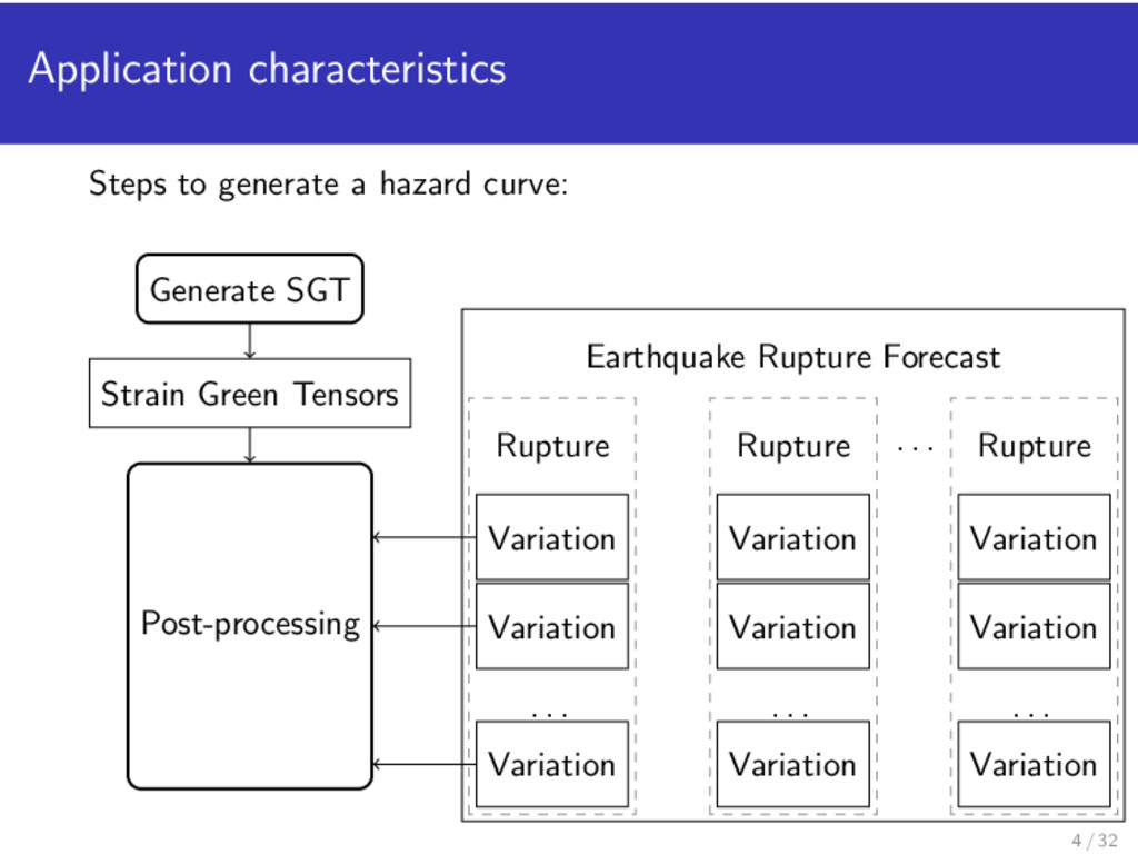
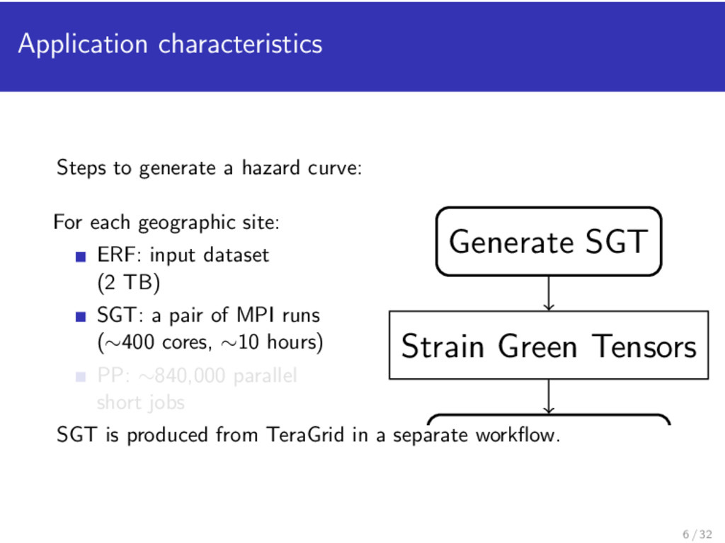
geographic site: ERF: input dataset (2 TB) SGT: a pair of MPI runs (∼400 cores, ∼10 hours) PP: ∼840,000 parallel short jobs Strain Green Tensors Generate SGT SGT is produced from TeraGrid in a separate workflow. 6 / 32
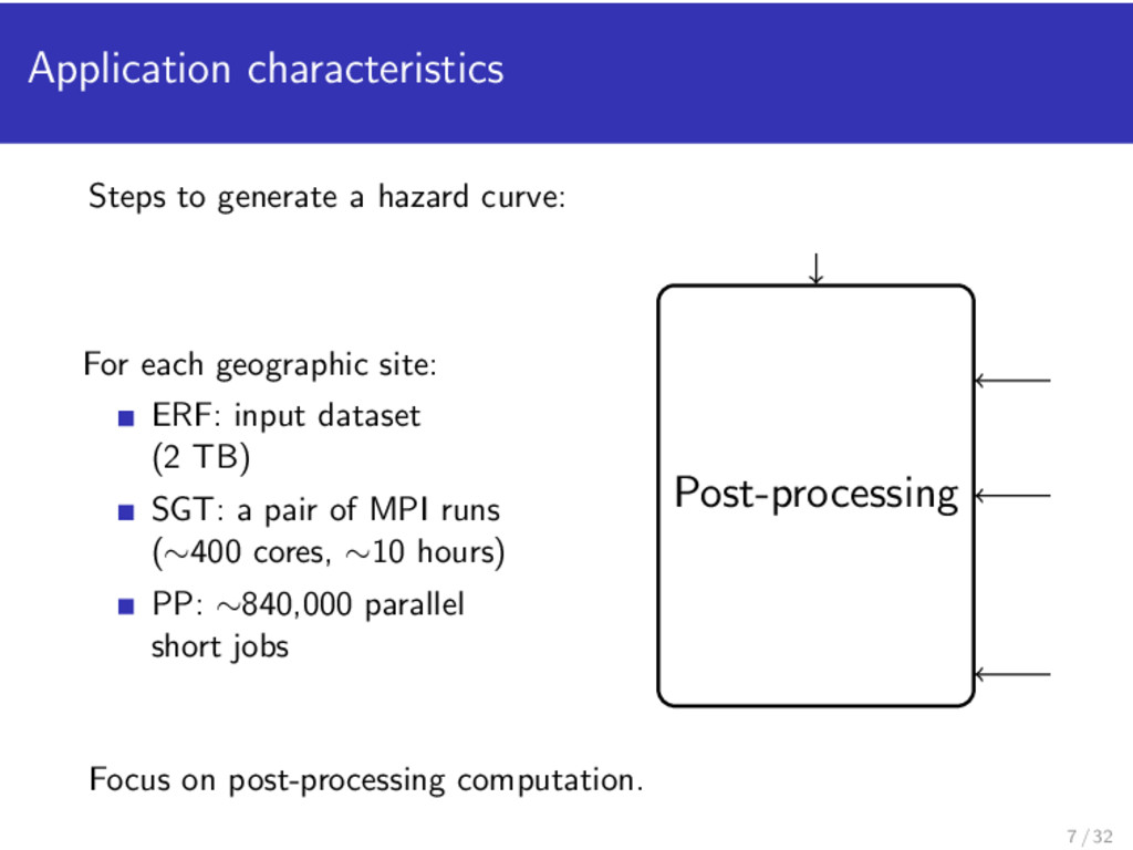
geographic site: ERF: input dataset (2 TB) SGT: a pair of MPI runs (∼400 cores, ∼10 hours) PP: ∼840,000 parallel short jobs Post-processing Strain Green Tensors Generate SGT V V V Focus on post-processing computation. 7 / 32
USC resources. Broaden access capability for the application. Expand access to OSG (opportunistic resource usage) Integration of TeraGrid and OSG resources using client tools Part of the NSF Extending Science Through Enhanced National Infrastructure (ExTENCI) project. 8 / 32
and distributed resources. Implicit task parallelism Automated data-flow dependency Handles backend operation. (Move files to/from and launch jobs to TG and OSG) We can change Swift as needed Apply application-specific lessons back to the engine Coaster multi-level scheduling (Pilot job mechanism) http://www.ci.uchicago.edu/swift swift 9 / 32
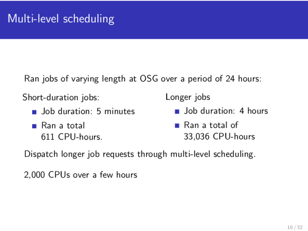
a period of 24 hours: Short-duration jobs: Job duration: 5 minutes Ran a total 611 CPU-hours. Longer jobs Job duration: 4 hours Ran a total of 33,036 CPU-hours Dispatch longer job requests through multi-level scheduling. 2,000 CPUs over a few hours 10 / 32
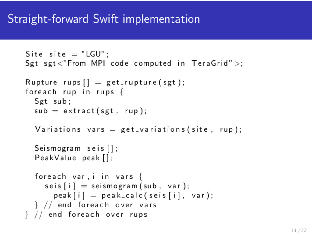
e = ”LGU”; Sgt sgt <”From MPI code computed i n TeraGrid ”>; Rupture rups [ ] = g e t r u p t u r e ( sgt ) ; f o r e a c h rup i n rups { Sgt sub ; sub = e x t r a c t ( sgt , rup ) ; V a r i a t i o n s v a r s = g e t v a r i a t i o n s ( s i t e , rup ) ; Seismogram s e i s [ ] ; PeakValue peak [ ] ; f o r e a c h var , i i n v a r s { s e i s [ i ] = seismogram ( sub , var ) ; peak [ i ] = p e a k c a l c ( s e i s [ i ] , var ) ; } // end f o re a c h over v a r s } // end f o r ea c h over rups 11 / 32
Pre-stage ERF dataset to a TeraGrid site For each location, generate SGT For each location, run PP Problem: need the full 2 TB on computing resource. OSG resources are opportunistic Disk quota limits on resources Swift currently does not have data-affinity-aware scheduling 12 / 32
Pre-stage ERF dataset to a TeraGrid site For each location, generate SGT For each location, run PP Problem: need the full 2 TB on computing resource. OSG resources are opportunistic Disk quota limits on resources Swift currently does not have data-affinity-aware scheduling 13 / 32
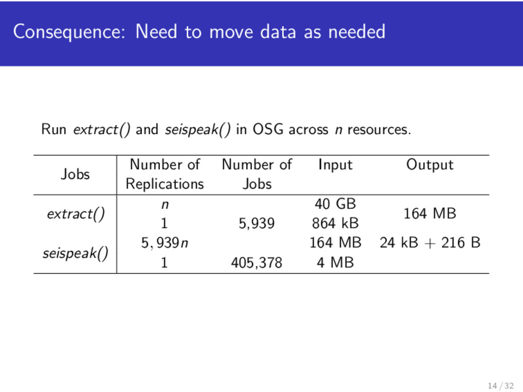
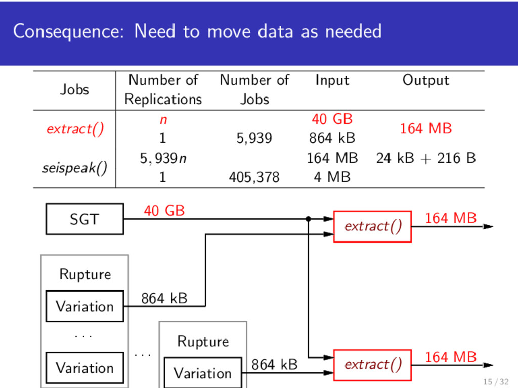
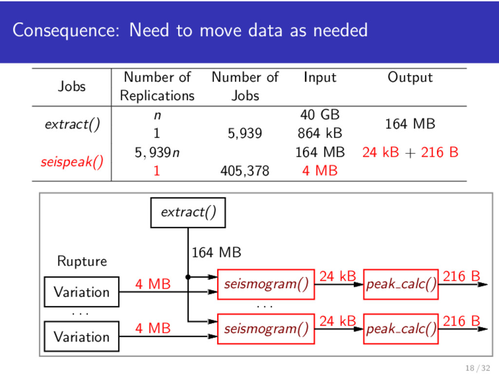
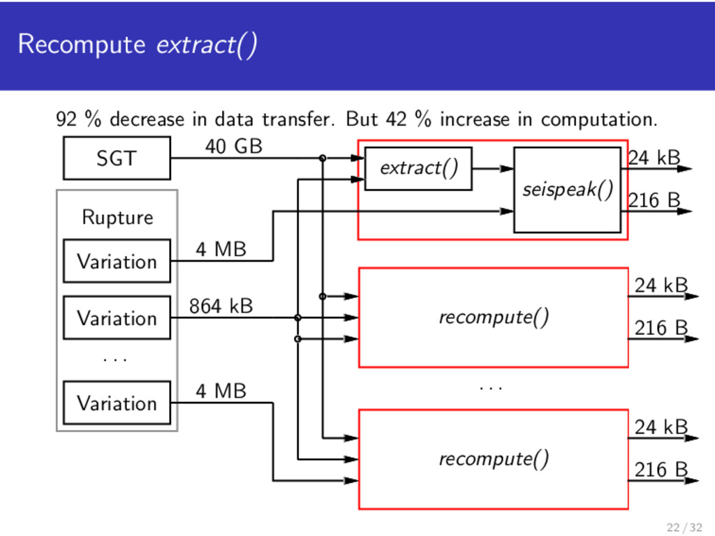
seispeak() in OSG across n resources. Jobs Number of Number of Input Output Replications Jobs extract() n 40 GB 164 MB 1 5,939 864 kB seispeak() 5, 939n 164 MB 24 kB + 216 B 1 405,378 4 MB 14 / 32
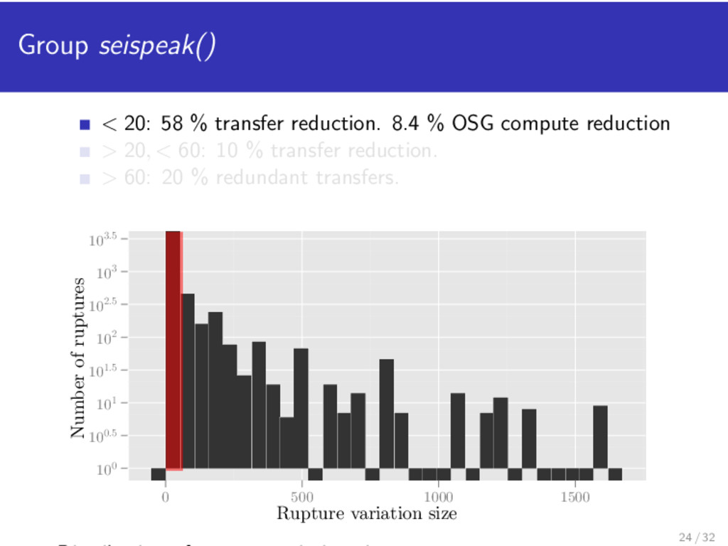
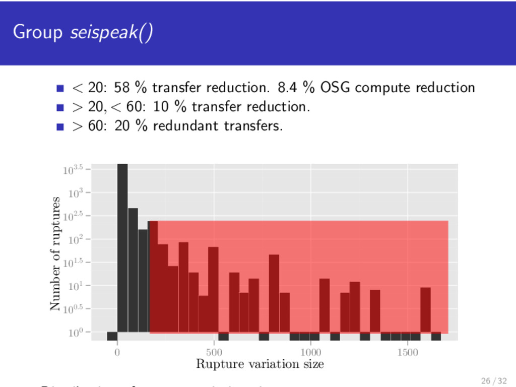
2,000 CPUs busy. Number of extract() seispeak() Resources (n) n = 1 205 MB/s 74 MB/s n = 20 3.7 GB/s 594 MB/s For n = 15, experimental result is 10 MB/s (extract()) and 5 MB/s (seispeak()) 19 / 32
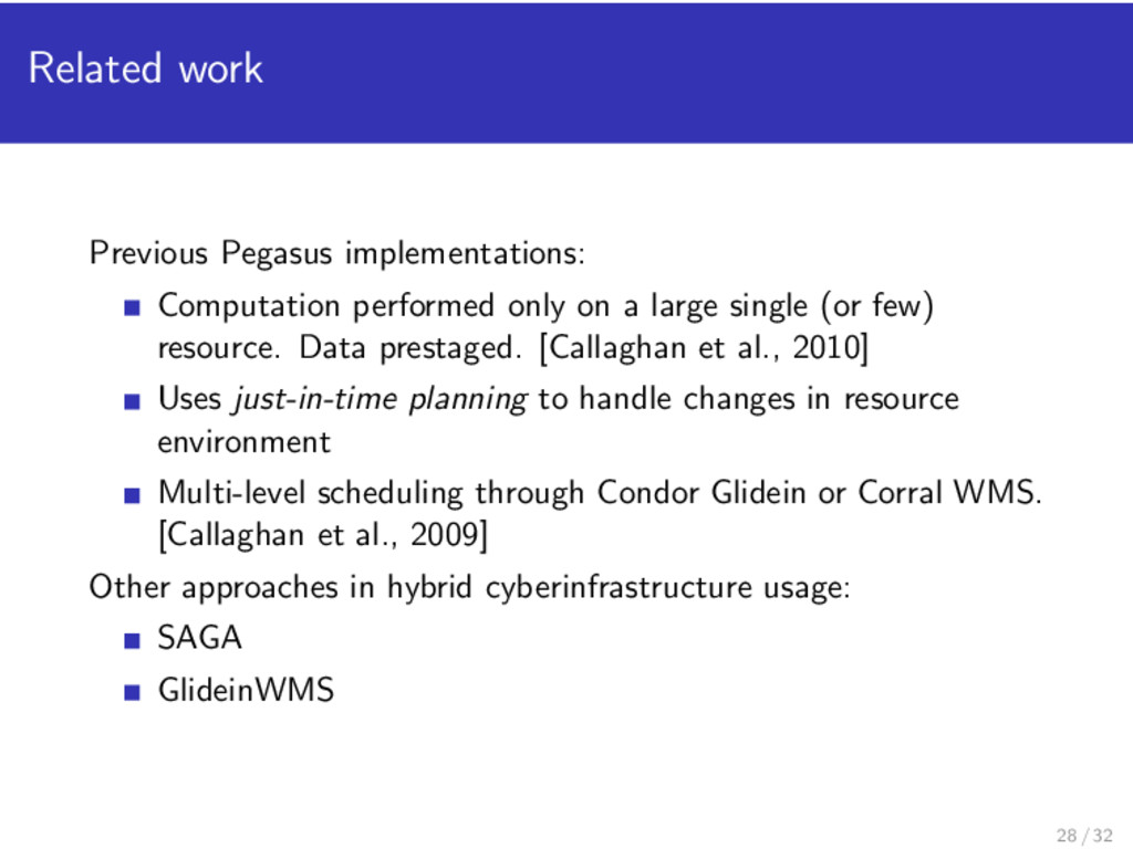
large single (or few) resource. Data prestaged. [Callaghan et al., 2010] Uses just-in-time planning to handle changes in resource environment Multi-level scheduling through Condor Glidein or Corral WMS. [Callaghan et al., 2009] Other approaches in hybrid cyberinfrastructure usage: SAGA GlideinWMS 28 / 32
models help in engineering the computation. Data movement as key performance issue Performance change by altering data movements and computation. 29 / 32
components Test workflow optimizations that minimize bandwidth. Data-aware scheduling on Swift Add other hazard-assessment models on the workflow 30 / 32
Maechling, C. Brooks, K. Vahi, K. Milner, R. Graves, E. Field, D. Okaya, and T. Jordan, “Scaling up workflow-based applications,” Journal of Computer and System Sciences, vol. 76, no. 6, p. 18, 2010. [Online]. Available: http://dx.doi.org/10.1016/j.jcss.2009.11.005 S. Callaghan, P. Maechling, E. Deelman, P. Small, K. Milner, and T. Jordan, “Many-Task Computing (MTC) Challenges and Solutions,” in Supercomputing 2009, 2009, poster. 32 / 32