Exo-Obs Course: Ultraviolet/X-ray Science and Atmospheric Escape

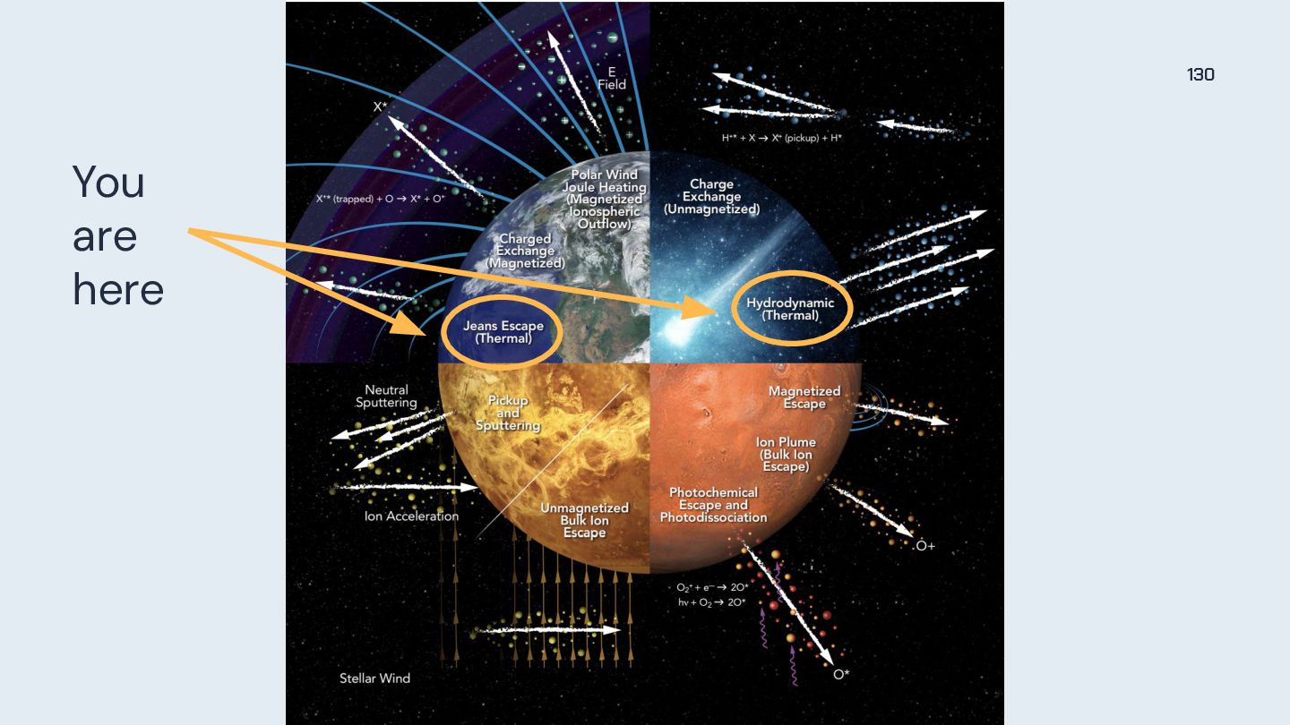
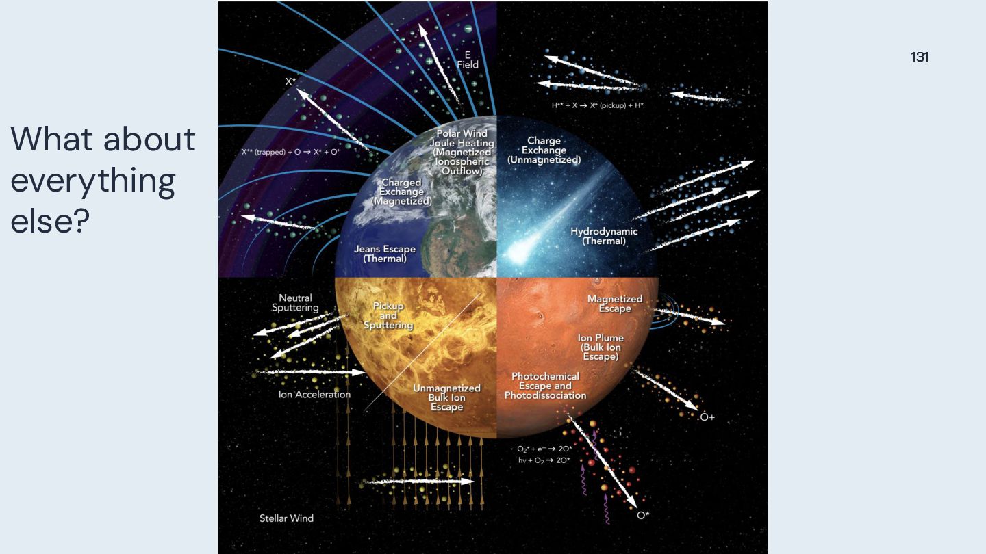
I will be sharing the slides I developed for a graduate level course on Exoplanets and Observational Astronomy. This is the sixth completed slide deck for this course. It covers topics on fundamentals of ultraviolet and x-ray astronomy as well as the effects of space weather on exoplanet atmospheres and atmospheric escape

The ultraviolet and x-ray technical slides were adapted from Jay Strader's graduate course elective on observational astronomy.

Transcript

1. UV/X-RAY & ATMOSPHERIC ESCAPE 1 Created by: Adina Feinstein
2. Relevant Readings Gronoff+2020 Parke Loyd+2025
3. UV ASTRONOMY 3 SLIDES ADAPTED FROM JAY STRADER
4. 4 Why use the ultraviolet (UV)? 1. Warm/hot objects have spectral energy distributions that peak in the ultraviolet.
5. 5 Why use the ultraviolet (UV)? 1. Warm/hot objects have spectral energy distributions that peak in the ultraviolet. 2. A lot of elements, including hydrogen and helium, have their strongest ground states at UV wavelengths.
6. 6 Why use the ultraviolet (UV)? 1. Warm/hot objects have spectral energy distributions that peak in the ultraviolet. 2. A lot of elements, including hydrogen and helium, have their strongest ground states at UV wavelengths. 3. UV uniquely traces common species from warm gas (~106K gas).
7. 7 Why use the ultraviolet (UV)? 1. Warm/hot objects have spectral energy distributions that peak in the ultraviolet. 2. A lot of elements, including hydrogen and helium, have their strongest ground states at UV wavelengths. 3. UV uniquely traces common species from warm gas (~106K gas). Problems with the UV 1. The UV is very sensitive to dust.
8. 8 Why use the ultraviolet (UV)? 1. Warm/hot objects have spectral energy distributions that peak in the ultraviolet. 2. A lot of elements, including hydrogen and helium, have their strongest ground states at UV wavelengths. 3. UV uniquely traces common species from warm gas (~106K gas). Problems with the UV 1. The UV is very sensitive to dust. 2. Restricted to space-based facilities only.
9. 9 UV Regimes Extreme UV 124 - 912 Å Opacity is high at these wavelengths. It is a very poorly studied wavelength range. Far-UV 912 - 2000 Å 912 Å corresponds to the wavelength of photons that are energetic enough to ionize H I. Near-UV 2000 - 3200 Å The limit is roughly due to the atmospheric cutoff.
10. 10 UV Detectors UV photons are more energetic than optical photons. One issue is that typical CCDs are too good, making it challenging to not have optical wavelength contamination in your UV CCD.
11. 11 UV Detectors The far-UV (FUV; 1150 - 1775 Å) arm of the Hubble Space Telescope/ Cosmic Origins Spectrograph (COS) has a “microchannel plate” detector.
12. 12 UV Microchannel Plate HST/COS is essentially an array of photomultiplier tubes. The NUV detectors are similar.
13. 13 UV Microchannel Plate HST/COS is essentially an array of photomultiplier tubes. The NUV detectors are similar. Photocathode converts Photon to electron.
14. 14 View of a Single Channel HST/COS is essentially an array of photomultiplier tubes. The NUV detectors are similar. Incoming UV photon
15. 15 UV Microchannel Plate HST/COS is essentially an array of photomultiplier tubes. The NUV detectors are similar. Microchannel plate amplifies the electron to 104-7.
16. 16 Advantages of Microchannel Plate • We can make microchannel plates that are “solar-blind” (i.e., they are only sensitive to specific wavelengths and are not contaminated by optical sunlight).
17. 17 Advantages of Microchannel Plate • We can make microchannel plates that are “solar-blind” (i.e., they are only sensitive to specific wavelengths and are not contaminated by optical sunlight). • We can count (“time-tag”) photons as they hit the detector (i.e., you can make light curves from a single exposure).
18. 18 Advantages of Microchannel Plate • We can make microchannel plates that are “solar-blind” (i.e., they are only sensitive to specific wavelengths and are not contaminated by optical sunlight). • We can count (“time-tag”) photons as they hit the detector (i.e., you can make light curves from a single exposure). • They are cheap to make and reliable to use in space.
19. 19 Advantages of Microchannel Plate • We can make microchannel plates that are “solar-blind” (i.e., they are only sensitive to specific wavelengths and are not contaminated by optical sunlight). • We can count (“time-tag”) photons as they hit the detector (i.e., you can make light curves from a single exposure). • They are cheap to make and reliable to use in space. • There is no readout noise.
20. 20 Available UV Facilities 1. Hubble Space Telescope: UV photometry and spectroscopy from ~900 - 3200 Å.
21. 21 Available UV Facilities 1. Hubble Space Telescope: UV photometry and spectroscopy from ~900 - 3200 Å. 2. Neil Gehrels Swift Observatory (Swift): Ultraviolet/Optical Telescope (UVOT) that operates at 1600 - 6000 Å. UVOT has spectroscopic capabilities from 1700 - 2900 Å.
22. 22 Available UV Facilities 1. Hubble Space Telescope: UV photometry and spectroscopy from ~900 - 3200 Å. 2. Neil Gehrels Swift Observatory (Swift): Ultraviolet/Optical Telescope (UVOT) that operates at 1600 - 6000 Å. UVOT has spectroscopic capabilities from 1700 - 2900 Å. 3. XMM-Newton: Optical Monitor (OM) provides simultaneous optical or UV photometry with X-ray spectroscopy.
23. 23 Available UV Facilities 1. Hubble Space Telescope: UV photometry and spectroscopy from ~900 - 3200 Å. 2. Neil Gehrels Swift Observatory (Swift): Ultraviolet/Optical Telescope (UVOT) that operates at 1600 - 6000 Å. UVOT has spectroscopic capabilities from 1700 - 2900 Å. 3. UltraViolet EXPlorer (UVEX): expected to launch in 2030.
24. 24 Archival UV Facilities 1. Galaxy Evolution Explorer (GALEX): two-band UV photometry in the FUV (1350-1759 Å) and NUV (1750 - 2800 Å).
25. 25 Archival UV Facilities 1. Galaxy Evolution Explorer (GALEX): two-band UV photometry in the FUV (1350 - 1759 Å) and NUV (1750 - 2800 Å). 2. Colorado Ultraviolet Transit Experiment (CUTE): small UV cubesat with low resolution NUV spectroscopic capabilities (2550 - 3300 Å).
26. 26 Archival UV Facilities 1. Galaxy Evolution Explorer (GALEX): two-band UV photometry in the FUV (1350 - 1759 Å) and NUV (1750 - 2800 Å). 2. Colorado Ultraviolet Transit Experiment (CUTE): small UV cubesat with low resolution NUV spectroscopic capabilities (2550 - 3300 Å). 3. Far Ultraviolet Spectroscopic Explorer (FUSE): R~20,000 with FUV wavelength coverage (905 - 1200 Å).
27. 27 Archival UV Facilities 1. Galaxy Evolution Explorer (GALEX): two-band UV photometry in the FUV (1350 - 1759 Å) and NUV (1750 - 2800 Å). 2. Colorado Ultraviolet Transit Experiment (CUTE): small UV cubesat with low resolution NUV spectroscopic capabilities (2550 - 3300 Å). 3. Far Ultraviolet Spectroscopic Explorer (FUSE): R~20,000 with FUV wavelength coverage (905 - 1200 Å). 4. International Ultraviolet Explorer (IUE): R~300-10,000 spectroscopic capabilities (1150 - 3200 Å).
28. 28 Future UV Facilities 1. UltraViolet EXPlorer (UVEX): similar to GALEX, in that it will have two wide-field imagers operating at FUV and NUV wavelengths. Expected to launch in 2030. .
29. 29 Future UV Facilities 1. UltraViolet EXPlorer (UVEX): similar to GALEX, in that it will have two wide-field imagers operating at FUV and NUV wavelengths. Expected to launch in 2030. 2. Habitable Worlds Observatory (HWO): TBD
30. X-RAY ASTRONOMY 30 SLIDES ADAPTED FROM JAY STRADER
31. 31 X-ray Regimes Hard X-rays 1-10+ keV < 12.4 Å Penetrate everything except very dense gas clouds. Soft X-rays 0.1 - 1 keV 12.4 - 124 Å Readily absorbed by the ISM.
32. 32 Why bother in the X-ray? Astronomers understood that X-rays would be easily absorbed by interstellar gas. Thus, it was not expected that X-rays would be astrophysically interesting and/or useful. The first X-ray detection was made using a sounding rocky in 1962. The rocket was attempting to image the Moon, and accidentally discovered the bright neutron star LMXB Sco X-1. Of course, now we know the X-ray is essential for understanding compact objects, hot gas, etc.
33. 33 Sources of X-rays 1. Optically thick thermal blackbody with T eff ≥ 106-7 K
34. 34 Sources of X-rays 1. Optically thick thermal blackbody with T eff ≥ 106-7 K 2. Optically thin thermal bremsstrahlung radiation, which is the primary cooling process for T gas ≥ 107 K
35. 35 Bremsstrahlung Radiation Bremsstrahlung radiation is produced by the deceleration of a charged particle when deflected by another charged particle. It guarantees that even very low-density plasmas will cool, although the cooling timescale will be longer.
36. 36 Sources of X-rays 1. Optically thick thermal blackbody with T eff ≥ 106-7 K 2. Optically thin thermal bremsstrahlung radiation, which is the primary cooling process for T gas ≥ 107 K 3. Sources of nonthermal radiation (e.g., synchrotron, inverse Compton)
37. 37 Synchrotron Radiation Synchrotron radiation occurs when a charged particle encounters a strong magnetic field and the particle is accelerated along the field line.
38. 38 Synchrotron Radiation Synchrotron radiation produces a photon distribution that is a power-law with an exponential cutoff.
39. 39 Synchrotron Radiation Synchrotron radiation is observed in shocks and jets: supernova remnants, energetic pulsars, accreting black holes, stellar atmospheres, coronal mass ejections
40. 40 Inverse Compton Inverse compton radiation occurs when a photon is upscattered by a relativistic electron. This generally occurs in accreting compact objects, jets, and other shocks. Inverse compton scattering can occur simultaneously with synchrotron radiation and is often hard to distinguish between. Electron Scattered photon Incident photon
41. 41 X-ray Regimes Hard X-rays 1-10+ keV < 12.4 Å Typically from nonthermal emission. Soft X-rays 0.1 - 1 keV 12.4 - 124 912 - 2000 Å Typically from thermal emission.
42. 42 X-ray Focusing X-rays don’t usually reflect like visible light because the refractive index of materials is usually slightly less than 1. Snell’s law predicts that most X-rays will refract into the material and get absorbed, rather than reflect. This makes using normal mirrors a problem.
43. 43 X-ray Focusing At very shallow (nearly grazing) angles, the X-rays cannot penetrate the surface efficiently. In this configuration, X-rays undergo total external reflection. This means that you can focus the X-rays, but only with grazing incidence mirrors of high surface densities. Missions like XMM-Newton and Chandra use gold and iridium.
44. 44 X-ray Focusing Just like in the optical, we need two reflections to correct aberrations for a decent field of view.
45. 45 X-ray Focusing The reflection off of a combination of two elements (a paraboloid followed by a hyperboloid) works better for X-ray astronomy
46. 46 X-ray Focusing Due to the low grazing incidence, typical focal lengths of X-ray facilities are long. ~10 m
47. 47 Hard X-ray Focusing The only focusing hard X-ray telescope (E > 10 keV) uses “Bragg reflection,” which relies on reflecting off of alternating layers of low and high density materials.
48. 48 X-ray Detectors Like some UV instruments, some X-ray facilities use a microchannel plate detector, which again is “simply” an array of photomultiplier tubes. The advantages are the same: • Can make them solar (optical) blind • Can time-tag photons • No readout noise • Cheap/reliable in space
49. 49 X-ray CCDs Some facilities use Si CCDs. When an X-ray photon interacts with the CCD, it is absorbed and produces a cloud of electrons. The number of photons generated is proportional to the photon’s energy. On average, 1 e- ~ 3.7 eV in a Si detector. E photon = N e x 3.7 eV Where N e is the number of electrons generated.
50. 50 X-ray Efficiency The efficiency of X-ray detection (“effective area”) is very energy-dependent. This translates to the efficiency of the blocking filter that is used within the instrument.
51. 51 Actually Detecting the X-ray X-ray astronomy often relies on the shell behavior of electrons close to the nucleus.
52. 52 Actually Detecting the X-ray On average, each ~3.7 eV energy produces 1 electron in Si, so each X-ray produces 100s-1000s of electrons. All of the produced electrons can be read out by the CCD and counted, yielding an estimate of the X-ray photon energy. The readout time is typically ≤ 3.2 seconds. This means that X-ray CCDs offer low-resolution (R~20-30) spectroscopy by default. How?
53. 53 X-ray CCD “spectroscopy” The low resolution spectroscopy that can be achieved with an X-ray CCD comes from the fact that the CCD can distinguish broad energy ranges. It cannot resolve fine spectral lines. The spectral resolving power: R ~ E/ΔE Where E is the photon energy and ΔE is the uncertainty on the energy.
54. 54 X-ray CCD “spectroscopy” - the dark side X-ray CCDs cannot distinguish between different incoming X-ray photons that hit in the same location within a ~3.2s integration window. This can produce a pileup, where two low-energy photons are misinterpreted as a single high-energy photon. This changes the apparent spectrum of the area. One way around this is the trade area for read-out speed to reduce the effects of pileups. Example of a bad pileup, that gave E > 12 keV - rejected by spacecraft.
55. 55 X-ray Background Noise is essentially irrelevant. The vast majority of X-ray photons come from real background X-ray sources, which can be resolved with sufficient exposure times.
56. 56 X-ray Spectroscopy Spectroscopy at R ≳ 1000 is possible through slitless transmission gratings. In x-ray astronomy, this is set by closely spaced series of gold bars. These gratings have low efficiency and can/should really only be used for bright targets.
57. 57 The Microcalorimeter A microcalorimeter is a thermal device made of an absorber, and thermistor (resistor that is highly dependent on temperature), and a heat sink.
58. 58 The Microcalorimeter The absorber must do three things:
59. 59 The Microcalorimeter The absorber must do three things: 1. Absorb X-rays efficiently
60. 60 The Microcalorimeter The absorber must do three things: 1. Absorb X-rays efficiently 2. Completely convert the absorbed energy into heat
61. 61 The Microcalorimeter The absorber must do three things: 1. Absorb X-rays efficiently 2. Completely convert the absorbed energy into heat 3. Have a low heat capacity
62. 62 The Microcalorimeter The absorber must do three things: 1. Absorb X-rays efficiently 2. Completely convert the absorbed energy into heat 3. Have a low heat capacity There is no material that is ideal for achieving all three of these objectives. In practice, deciding on the material of the absorber relies on striking a balance between these three properties. An example absorber is HgTe (mercury-telluride, which has good thermalizing properties and low heat capacity.
63. 63 The Microcalorimeter The thermistor/thermometer is a device that changes its electrical resistance with a small change in temperature. It is a sort-of thermometer.
64. 64 The Microcalorimeter The combination of the absorber and the thermistor is typically referred to as the “detector” in a microcalorimeter.
65. 65 The Microcalorimeter The heat sink absorbs heat from the detector, keeping it cool.
66. 66 The Microcalorimeter - How it works An X-ray photon hits the absorber, knocking an electron loose from an atom of the absorber material.
67. 67 The Microcalorimeter - How it works An X-ray photon hits the absorber, knocking an electron loose from an atom of the absorber material. The photoelectron rattles around in the absorber, ultimately raising the temperature of the absorber by ~mK.
68. 68 The Microcalorimeter - How it works An X-ray photon hits the absorber, knocking an electron loose from an atom of the absorber material. The photoelectron rattles around in the absorber, ultimately raising the temperature of the absorber by ~mK. The temperature-sensitive thermistor detects the temperature increase and equilibrates with the new temperature of the absorber.
69. 69 The Microcalorimeter - How it works The temperature increase in the thermistor is roughly proportional to the energy of the X-ray photon: ∆T ~ E/C ∆T is the change in temperature E is the energy of the X-ray C is the heat capacity of the absorber
70. 70 The Microcalorimeter - How it works The thermistor begins to cool as the heat flows from the detector to the heat sink.
71. 71 The Microcalorimeter - How it works The thermistor begins to cool as the heat flows from the detector to the heat sink. The thermistor returns to its normal operating temperature.
72. 72 Hitomi X-ray Calorimeter Launched: February 17, 2016 Mission end: March 26, 2016 Hitomi had lost attitude control and broke into ~10 pieces. Was exciting for about a month!
73. 73 Hitomi Successor: XRISM Launched: September 6, 2023 A protective shutter over one of the instrument detectors has failed to open, limiting the observations to > 1.8 keV, as opposed to the planned 0.3 eV.
74. 74 Optical vs. X-ray Optical The fundamental thing we observe is an image. X-ray
75. 75 Optical vs. X-ray Optical The fundamental thing we observe is an image. X-ray The fundamental thing observed is not an image. What is it?
76. 76 Optical vs. X-ray Optical The fundamental thing we observe is an image. X-ray The fundamental thing observed is not an image. What is it? A photon (“event”) list: lots of parameters per photon typically represented by 2D position, time, and energy
77. 77 Optical vs. X-ray Optical We have lots of photons and proper treatment of the background is important. X-ray
78. 78 Optical vs. X-ray Optical We have lots of photons and proper treatment of the background is important. X-ray We have very few photons. But, ech X-ray photon has ~100x energy of an optical photon!
79. 79 Optical vs. X-ray Optical We have lots of photons and proper treatment of the background is important. X-ray We have very few photons. But, ech X-ray photon has ~100x energy of an optical photon! X-ray telescopes have small effective areas (<< 1 m2) and backgrounds don’t usually matter.
80. 80 X-ray Statistics When working with X-ray data, you will almost always be in the low N regime, where Poisson statistics reign. E.g. 9 counts is considered a strong detection. 3-4 counts is “believable.”
81. 81 X-ray Analysis The instrument response function is complex. Typical X-ray astronomy analysis relies on forward modeling the data. This means that you convolve a model with the response of the instrument and fit that to the data, rather than the reverse (similar to transmission spectra sometimes!).
82. 82 X-ray Analysis The instrument response function is complex. Typical X-ray astronomy analysis relies on forward modeling the data. This means that you convolve a model with the response of the instrument and fit that to the data, rather than the reverse (similar to transmission spectra sometimes!). There is lots of funding for X-ray data analysis software. The methods are relatively well-developed and standardized at this point.
83. 83 X-ray Analysis The instrument response function is complex. Typical X-ray astronomy analysis relies on forward modeling the data. This means that you convolve a model with the response of the instrument and fit that to the data, rather than the reverse (similar to transmission spectra sometimes!). There is lots of funding for X-ray data analysis software. The methods are relatively well-developed and standardized at this point. It is common to use archival data.
84. 84 Quantifying an X-ray “Detection” Congratulations! You detected 6 X-ray photons at the expected location of your object. Assume the background contribution is ~ 1 photon. What is the significance of your detection? √N photons not √N photons
85. 85 Quantifying an X-ray “Detection” Congratulations! You detected 6 X-ray photons at the expected location of your object. Assume the background contribution is ~ 1 photon. What is the significance of your detection? √N photons not √N photons
86. 86 Quantifying an X-ray “Detection” Congratulations! You detected 6 X-ray photons at the expected location of your object. Assume the background contribution is ~ 1 photon. What is the significance of your detection? Instead, you want to evaluate the probability of observing 6 photons assuming the rate is 0 photons and the background is 1 photon. √N photons not √N photons
87. 87 Quantifying an X-ray “Detection” The probability, P, of N events occurring depending on the mean number, μ, that is expected. N is an integer. μ is real. Distribution
88. 88 Quantifying an X-ray “Detection” If you detect 6 photons and the background is 1 photon, how many watermelons did Steve get from the supermarket?
89. 89 Quantifying an X-ray “Detection” If you detect 6 photons and the background is 1 photon, you detected 5 photons from the source. Assuming the source should have 0 photons, P(S=0) ~ 0.0005, which is ≥ 3σ.
90. 90 Quantifying an X-ray “Detection” If you detect 4 photons and the background is 1 photon, you detected 3 photons from the source. Assuming the source should have 0 photons, P(S=0) ~ 0.02, which is ~2σ.
91. 91 Quantifying an X-ray “Detection” If you detect 2 photons and the background is 3 photons, P(S=0) ~ 0.59, which is still more likely than not that the source was detected, but it’s not significant.
92. 92 The Units of X-ray X-ray fluxes are typically expressed in physical units, unlike optical astronomy (e.g., erg s-1 cm-2). X-ray fluxes are always integrated over some bandpass (e.g., 0.3-8 keV). Sometimes you will see the flux expressed in units of Crab Nebula, the equivalent to Vega in the optical. 1 mCrab (0.5-10 keV) ~ 4 x 10-11 erg s-1 cm-2.
93. 93 X-ray Cheat Sheet Chandra, XMM-Newton: best imaging telescopes. Chandra has better spatial resolution than XMM, while XMM has better sensitivity. Swift/XRT: easiest to get a quick observation. It is very good for monitoring, but it’s sensitivity is ~⅓ that of Chandra. NuSTAR: the only focusing hard X-ray instrument NICER: located on the International Space Station, best for timing, very low spatial resolution (does not image)
94. SPACE WEATHER 94
96. 96 The challenges Understanding planetary atmospheric escape is an interdisciplinary effort that is currently dominated by uncertainties. However, it is a very important field of study if we are to understand: 1. How stars interact with their planets 2. How planets evolve 3. The habitable conditions of rocky planets
97. 97 The challenges Understanding planetary atmospheric escape is an interdisciplinary effort that is currently dominated by uncertainties. However, it is a very important field of study if we are to understand: 1. How stars interact with their planets 2. How planets evolve 3. The habitable conditions of rocky planets It requires a significant amount conversation between heliophysics, astronomy, planetary science, and astrobiology.
98. 98 The challenges Understanding planetary atmospheric escape is an interdisciplinary effort that is currently dominated by uncertainties. However, it is a very important field of study if we are to understand: 1. How stars interact with their planets 2. How planets evolve 3. The habitable conditions of rocky planets It requires a significant amount conversation between heliophysics, astronomy, planetary science, and astrobiology.
100. 100 Recent Findings from the KISS Workshop Finding: The impacts of the local stellar particle environment on orbiting planets depends on a complex set of factors, many of which are poorly characterized, including planetary atmospheric composition, stellar and planetary magnetic fields, and the system’s evolutionary stage.
101. 101 Recent Findings from the KISS Workshop Finding: The impacts of the local stellar particle environment on orbiting planets depends on a complex set of factors, many of which are poorly characterized, including planetary atmospheric composition, stellar and planetary magnetic fields, and the system’s evolutionary stage. Ways to go: 1. Model long-term atmospheric evolution under varied space weather conditions 2. Observing atmospheric escape driven by non-thermal processes (e.g. coronal mass ejections) 3. Assessing how space weather may trigger or suppress conditions favorable to life.
102. 102 Recent Findings from the KISS Workshop Finding: No current observatory has been purpose-built to observe stellar particle environments. As a result, our constraints on key phenomena like stellar winds and coronal mass ejections remain speculative, often relying on instruments not designed for these detections or solar observations.
103. 103 Recent Findings from the KISS Workshop Finding: No current observatory has been purpose-built to observe stellar particle environments. As a result, our constraints on key phenomena like stellar winds and coronal mass ejections remain speculative, often relying on instruments not designed for these detections or solar observations. Ways to go: Prioritize the design and development of instruments explicitly optimized for detecting stellar particle events (e.g., radio, UV, and X-ray): 1. High-contrast imaging for stellar coronae and winds 2. Low-frequency radio arrays for stellar eruption bursts 3. UV/X-ray spectrographs to track coronal activity
104. 104 Recent Findings from the KISS Workshop Finding: The study of stellar energetic particles and coronal mass ejections is in its infancy. These phenomena are difficult to detect directly, but multiple indirect observational signatures, validated against the Sun, could open paths to studying them in other stars.
105. 105 Recent Findings from the KISS Workshop Finding: The study of stellar energetic particles and coronal mass ejections is in its infancy. These phenomena are difficult to detect directly, but multiple indirect observational signatures, validated against the Sun, could open paths to studying them in other stars. Ways to go: 1. Coordinated multiwavelength campaigns to capture transient space weather events 2. Comparative analyses across stellar types to identify scaling relations and trends
106. 106 Recent Findings from the KISS Workshop Finding: Progress in exospace weather science requires sustained, deliberate investment in coordinates observational infrastructure. Existing facilities lack the sensitivity, cadence, or spectral coverage needed to characterize particle and magnetic environments or to capture key time-domain phenomena across diverse stellar types.
107. 107 Recent Findings from the KISS Workshop Finding: Progress in exospace weather science requires sustained, deliberate investment in coordinates observational infrastructure. Existing facilities lack the sensitivity, cadence, or spectral coverage needed to characterize particle and magnetic environments or to capture key time-domain phenomena across diverse stellar types. Ways to go: 1. Leverage synergies across space-and ground-based observatories and wavelengths 2. Enable long-duration time-domain monitoring of active and representative stellar populations 3. Integrating exospace weather objectives into mission design and science traceability matrices from the earliest planning stages
108. 108 The role of energetic particles A particle’s characteristic energy will generally determine the depth to which the particle can penetrate a planet’s atmosphere.
109. 109 The role of energetic particles - Solar Wind The solar wind is mostly comprised of ions and electrons with energies of the order of keV. These particles mostly affect the upper atmosphere. They serve as a source of ionization and dissociation, which leads to chemical reactions and non-thermal atmospheric escape processes.
110. 110 The role of energetic particles - Solar Wind If there is a crustal magnetic field (i.e. Earth), the solar wind particles can get accelerated and enhances the energy released into the upper layer of the atmosphere.
111. 111 The role of energetic particles - Solar Energetic Particles Solar energetic particles (SEPs) have energies in the MeV-GeV range. These particles can penetrate to the mesosphere.
112. 112 The role of energetic particles - Solar Energetic Particles SEPs ionize species in the mesosphere, which then rapidly recombine, driving nonthermal chemistry. Nonthermal chemistry includes the creation of hazes and, in some cases, “prebiotic molecules” that may play a role in biogenesis.
113. 113 The role of energetic particles - Galactic Cosmic Rays Galactic cosmic rays (GCRs) that interact with planets have energies in the GeV-TeV range. GCRs can penetrate down to the lower stratosphere and all the way to the surface (at least for Earth).
114. 114 The role of energetic particles - Galactic Cosmic Rays GCRs ionize molecules, modify chemistry, and serve as a damaging source of radiation. Fortunately, the rate of GCRs is too low to pose a serious hazard to life. It is unclear what the long term effect of GCRs are.
115. 115 How do we detect the effects of space weather? The “obvious” answer: Space weather erosion of atmospheres can be detected by the lack of atmosphere, when one is otherwise expected to be there.
116. 116 How do we detect the effects of space weather? The “obvious” answer: Space weather erosion of atmospheres can be detected by the lack of atmosphere, when one is otherwise expected to be there. Why is this not actually obvious (for rocky planets)?
117. 117 How do we detect the effects of space weather? The “obvious” answer: Space weather erosion of atmospheres can be detected by the lack of atmosphere, when one is otherwise expected to be there. Why it’s not obvious: Quantifying the role of space weather in the removal of an atmosphere requires a firm understanding and firm constraints on geological outgassing, initial volatile reservoir, and how these properties change across different planets.
118. 118 Thermal Atmospheric Escape The retention of primordial gas envelopes (e.g. the amount of hydrogen and helium a planet accretes during formation) is dependent on the (thermal) hydrodynamic escape driven primarily by the stellar extreme-UV and X-ray (XUV) radiation.
119. 119 Jeans Regime Assuming the neutral atmospheric constituents in the upper atmosphere are in local thermodynamic equilibrium, the escape flux is given as: Gronoff et al. (2020) N i = total number of particles u i = the thermal speed for species i λ ex = the Jeans parameter (the ratio of the gravitational energy to thermal energy)
120. 120 Jeans Regime Assuming the neutral atmospheric constituents in the upper atmosphere are in local thermodynamic equilibrium, the escape flux is given as: Gronoff et al. (2020) This is a relatively good approximation for the thermal escape when the atmosphere is strongly gravitationally bound to the planet. This formulation holds true for all constituents of the atmosphere independently, and can be evaluated down to the exobase.
121. 121 Jeans Regime The exobase is where the mean free path of the ith constituent is equal to the scale height, H, (i.e. essentially collisionless) . While the Jeans parameter is the main parameter of thermal escape, the location of the exobase is extremely important. In some cases (e.g., Titan), the altitude of the exobase is non-negligible compared to the radius of the planet. While the flux per unit surface is small, it can become an important source of mass loss when taking the entire exobase surface into account. Gronoff et al. (2020)
122. 122 Gronoff et al. (2020) In the case where the internal energy of individual gas molecules approaches the kinetic escape velocity, the gas will begin to escape as a flow of continuous fluid. How does this differ from Jeans atmospheric escape? Hydrodynamic Regime
123. 123 In the case where the internal energy of individual gas molecules approaches the kinetic escape velocity, the gas will begin to escape as a flow of continuous fluid. How does this differ from Jeans atmospheric escape? Collisional considerations Gronoff et al. (2020) Jeans “Collisionless”: the atmosphere is not only retained by the gravitational pull on individual molecules but also by the effective force of collision with other atmospheric molecules. Hydrodynamic Regime
124. 124 In the case where the internal energy of individual gas molecules approaches the kinetic escape velocity, the gas will begin to escape as a flow of continuous fluid. How does this differ from Jeans atmospheric escape? Collisional considerations Gronoff et al. (2020) Jeans “Collisionless”: the atmosphere is not only retained by the gravitational pull on individual molecules but also by the effective force of collision with other atmospheric molecules. Hydrodynamic “Collisional”: Molecules are so energetic that collisions are insufficient to restrict escape. The escaping flow of lighter gases is capable of exerting an effective force and dragging heavier molecules. Hydrodynamic Regime
125. 125 Hydrodynamic Regime Gronoff et al. (2020) In the case where the internal energy of individual gas molecules approaches the kinetic escape velocity, the gas will begin to escape as a flow of continuous fluid. N = number of molecules T e = temperature m = mass of the molecule
126. 126 Determining your Regime Gronoff et al. (2020) The regime of thermal escape is governed by the Jeans parameter. There is a critical value for λ ex below which there is a transition to hydrodynamic escape. This division is determined by the heat capacity ratio, which is directly linked to the degree of freedom of the molecule/atom. For an atmosphere dominated by H 2 , the division occurs at λ ex = 2.5.
127. 127 The Cosmic Shoreline The cosmic shoreline is a relationship between the XUV irradiation, I, from the host star and the escape velocity of the planet, v esc . For the solar system, this goes as I ∝ v esc 4 Zahnle & Catling (2017)
128. 128 The Cosmic Shoreline What is a limitation to the cosmic shoreline? Zahnle & Catling (2017)
129. 129 Nonthermal Escape on Rocky Planets The long-term evolution of outgassed, secondary atmospheres can be substantially affected by the strength of nonthermal processes. E.g., Atmospheric mass loss driven by stellar winds could completely strip away outgassed atmospheres. This has been simulated for the TRAPPIST-1 planets (Dong et al. 2018). In reality, it depends on the relative strength between the particle-drive atmospheric loss and the geological processes that could replenish the atmosphere (Krissansen-Totton, 2023).
130. 130 You are here
131. 131 What about everything else?
132. 132 Do magnetic fields protect planetary atmospheres from escape? Yes No
133. 133 Do magnetic fields protect planetary atmospheres from escape? Yes No
134. 134 Do magnetic fields protect planetary atmospheres from escape? Yes - Can protect from specific kinds of escape (e.g. ion sputtering) No
135. 135 Do magnetic fields protect planetary atmospheres from escape? No - What about Venus? It has a thick atmosphere, yet has a very weak magnetic field. Yes - Can protect from specific kinds of escape (e.g. ion sputtering)
136. 136 Aeronomy The escape rates have been seen to change as a function of the solar cycle. This is referred to as aeronomy, because it focuses on the evolution of the upper atmosphere.
137. 137 Aeronomy This can be easily seen in solar system planets. This figure summarizes the in-situ measurements of heavy ion escape rates from Venus, Earth, and Mars. Ramstad & Barabash (2021)
138. 138 Aeronomy Levine et al. (2024) It is much harder to look for this kind of behavior in other systems, but there has been some tentative evidence in the WASP-69 system.
139. 139 Atmospheric Chemistry High-energy particles impact the atmospheres (and surfaces) of terrestrial planets in the Solar System. For example, on Earth, high-energy particles can break apart N 2 , resulting in the formation of NO X species that destroy ozone through different reactions. Particles also dissociate forming HO X species, which are highly reactive and deplete both O 3 and CH 4 .
140. 140 Flare-Driven Chemistry - Instantaneous Effects Flare photons do not necessarily affect the amount of ozone. However, the NO X produced by high-energy photons (> 10 eV; λ < 124 nm) depleted almost all the ozone two years after the flare. The atmosphere recovered 50 years later… Segura et al. (2010)
141. 141 Flare-Driven Chemistry - Global view Chen et al. (2021) G star
142. 142 Flare-Driven Chemistry - Global view Chen et al. (2021) K star
143. 143 Flare-Driven Chemistry - Global view Chen et al. (2021) M star
144. 144 Flare-Driven Chemistry - Observables Chen et al. (2021)
145. 145 Aurorae When energetic particles precipitate into the magnetospheres and upper atmospheres of planets, it generates emission from UV to radio wavelengths.
146. 146 Aurorae - Magnetic Fields Magnetic fields can play an important role in the generation of aurorae. Electrons precipitating at Earth are more energetic than particles of the solar wind. This increase in energy is due to the interaction of the solar wind plasma and the magnetosphere. The magnetosphere is the region of space surrounding the planet where the magnetic field is dominant against incoming energetic particles.
147. 147 Aurorae - Magnetic Fields Magnetic fields can play an important role in the generation of aurorae. Electrons precipitating at Earth are more energetic than particles of the solar wind. This increase in energy is due to the interaction of the solar wind plasma and the magnetosphere. Mechanisms for the increased energy of particles in the magnetosphere include: magnetic reconnection, electromagnetic waves, and field-aligned currents.
148. 148 Magnetic Fields - Radio Emission Magnetic fields also play a key role in the generation of radio emission, as particles bound to generate aurorae travel along those field lines. The emission generated by these energetic particles arises through the electron cyclotron maser instability (ECMI). This mechanism is present in nearly all Solar System planets.
149. 149 Do aurora imply the presence of a magnetic field? Yes No
150. 150 Do aurora imply the presence of a magnetic field? Yes No
151. 151 Do aurora imply the presence of a magnetic field? A planet does not need to have an intrinsic magnetic field to produce auroral-like emission. E.g. - Venus shows that solar wind particles can be diverted towards the nightside of the planet and lead to auroral phenomena. This is due to the induced magnetic field generated in Venus’ ionosphere (upper atmosphere). It can be assumed that any plant with an ionosphere undergoes similar processes.
152. 152 Magnetic Fields - On Exoplanets Shkolnik et al. (2005); Cauley et al. (2019)
153. STELLAR MAGNETIC FIELDS 153
154. 154 What we can learn from the Sun We can observe modulation of the particle space weather around the Sun due to its magnetic activity cycle. XUV emission, flares, coronal mass ejections, and SEPs are all connected (either directly or indirectly) to the Sun’s magnetic field. McComas et al. (2008)
155. 155 What we know about other stars XUV emission, flares, coronal mass ejections, and SEPs McComas et al. (2008)
156. 156 What we know about other stars We can place observational constraints on the large-scale magnetic field structure of other main sequence stars through Zeeman-Doppler Imaging.
157. 157 Zeeman-Doppler Imaging: An aside You have a rotating star. Consider two magnetic spots of opposite polarities and different Doppler shifts on the surface. The spectral coordinates are at X 1 and X 2 . Carter et al. (1996)
158. 158 Zeeman-Doppler Imaging: An aside The intensity spectrum, I, associated with the two-spot group consists of two absorption profiles (1 per spot) centered on X 1 and X 2 . Carter et al. (1996)
159. 159 Zeeman-Doppler Imaging: An aside Through the Zeeman effect (splitting of spectral lines into several components in the presence of a magnetic field), each spot induces a small opposite shift of the line at I ± V, where V is the Stokes circular polarization parameter. Carter et al. (1996)
160. 160 Zeeman-Doppler Imaging: An aside By subtracted the right-handed from the left-handed circular polarisation spectra, the lines no longer cancel each other out as they would in a non-rotating star. Carter et al. (1996)
161. 161 Zeeman-Doppler Imaging: An aside The shape of the Stokes V profile informs us about the location of the magnetic spots on the visible stellar disk. Carter et al. (1996)
162. 162 Spectropolarimeters A spectropolarimeter is a combined spectrograph and polarimeter to measure how plane-polarized light is rotated across different wavelengths. Instrument Telescope Diameter [m] Spectral Resolution Wavelength Coverage [nm] ESPaDOnS at CFHT 3.6 65,000 370-1050 SPIRou at CFHT 3.6 70,000 980-2350 HARPSpol at ESO 3.6 115,000 378-907 PEPSI at LBT 2 x 8.4 220,000 383-907 CRIRES at VLT 8.2 100,000 950-5500
163. 163 What we know about other stars An overview of observational constraints on the large-scale magnetic field structure of cool main sequence stars. Sizes = relative strength of the magnetic field. Color = geometry of the field (red = poloidal; blue = toroidal) Shape = symmetry level (decagons = axisymmetric; star = non-axisymmetric)
164. 164 Stellar Magnetic Field Relationships Period-mass diagram of stars, where the color/size represents the strength of the magnetic field. The gray points are a sample of stars with known rotation periods, but no measured magnetic fields.
165. ATMOSPHERIC ESCAPE 165
168. 168 Exoplanet Outflows The hydrodynamic outflow of escaping planetary atmospheric material can be shaped by the stellar wind. This can be seen as the planet transits.
169. 169 Exoplanet Outflows The resulting light curve will show evidence of a tail of the escaping material. This example is for a hot Jupiter at a = 0.15 AU from a sun-like star. Owen et al. (2023)
170. 170 Signatures of Outflows: Lyman-α (1215.67 Å) Lyman-α traces the 1s-2p transition of hydrogen. Neutral hydrogen is the primary constituent of escaping atmospheres in most H 2 -dominated exoplanets. Lyman-α is the most sensitive tracer to neutral hydrogen in the upper atmosphere. Thus, observing an excess in Lyman-α absorption during a transit probes the escaping hydrogen.
171. 171 Signatures of Outflows: Lyman-α (1215.67 Å) By measuring the depth and shape of Lyman-α transits, one can constrain: • Neutral hydrogen column density • Outflow velocity • Total mass-loss rate
172. 172 Signatures of Outflows: Lyman-α (1215.67 Å) Cons: Interstellar H I absorption obscures the line core of Lyman-α, limiting our ability to only constraining the outflow from the wings of the line. Also, we cannot observe Lyman-α from the ground, limiting our observations to space observatories only. Vidal-Madjar et al. (2003)
173. 173 Lyman-α Detections This is the first detection of a Lyman-α outflow from HD 209458 (a hot Jupiter). These observations were taken with HST Vidal-Madjar et al. (2003)
174. 174 Lyman-α Detections Lyman-α outflows have also been detected on HD 189733 b. Lecavelier des Etangs et al. (2010); Bourrier et al. (2013)
175. 175 He I 1083 nm Metastable Triplet He I at 1083 nm traces the transition from 23S - 23P of neutral helium. Similarly to Lyman-α, it is sensitive to the upper atmosphere and outflows of neutral He. He I is very sensitive to the XUV because it is formed. This transition is metastable, meaning it cannot decay quickly to the ground state because the transition is forbidden.
176. 176 He I 1083 nm Metastable Triplet h𝜈 XUV has to have an energy > 24.6 eV to ionize the helium. The helium then recombines with an electron, leading to He in multiple excited states.. Some fraction of these recombinations will end up in the metastable state: An XUV photon comes in and ionizes the neutral helium: Oklopčić et al. (2018)
177. 177 He I 1083 nm Metastable Triplet The He I is very sensitive to the XUV photoionization rate from the host star. This is because when more He+ ions are produced, the more recombinations occur, increasing the abundance of He I in the metastable population. In theory, He I will change depending on the XUV flux of the host star (e.g., flares, activity cycles).
178. 178 He I Transit Observations WASP-69b Vissapragada et al. (2020); Zhang et al. (2022); Vissapragada et al. (2024) WASP-52b HD 189733 b TOI-1420 b
179. 179 He I Transit Observations Vissapragada et al. (2021) Why haven’t we confidently detected He I in young planets, whose stars have enhanced XUV flux?
180. 180 He I Stellar Variability Krolikowski et al. (2024) Monitoring the long-term time-averaged He variability as a function of age revealed that this line is very variable for young stars. Top: Median absolute value of He EW. Bottom: Estimate of the intrinsic variability of He EW
182. 182 Title
183. 183 Title
184. 184 Title
185. 185 Summary Table Process Origin Key Parameters Jeans Escape Temperature accelerates particles above the escape velocity T, g, λ ex > 2.5 Hydrodynamic escape Thermal acceleration, but the gas behaves like a fluid T, g, λ ex < 2.5 Photochemical/Ion recombination Ion recombination releases kinetic energy Low g, ion species, requires ionosphere densities Dissociation Molecular photodissociation releases kinetic energy Low g, requires atmospheric densities Ion pickup Solar wind picks up ions from ionosphere Requires compressed/no magnetosphere Ion sputtering Accelerated ions from the ionosphere translates their kinetic energy B, Requires compressed/no magnetosphere Gronoff et al. (2020)
186. 186 Summary Table Process Origin Key Parameters Charge exchange - trapped Fast ion trapped in magnetosphere becomes ENA through charge exchange Requires magnetosphere, ion density and temperature, neutral densities Charge exchange - solar wind Solar wind ion becomes ENA that can access thermosphere and increases heating Requires large coronae Charge exchange - particle precipitation Particle precipitating in thermosphere becomes ENA and translate kinetic energy Requires precipitation fluxes, cross sections Ionospheric outflow Creation of ion upward wind through ambipolar diffusion Requires magnetic fields, ionosphere Other Plasma instabilities leading to ions going upwards and being picked by the solar wind Requires magnetic fields, ion density and temperature Gronoff et al. (2020)
187. 187 How do we detect the effects of space weather? Observational Signature Solar System Planets Exoplanets Aurorae Possible but not yet observed through radio observations Nonthermal atmospheric escape Atmospheric outflows Stripped secondary atmospheres Chemical perturbations Surface Space Weathering