Exo-Obs Course: Exoplanet Atmospheres

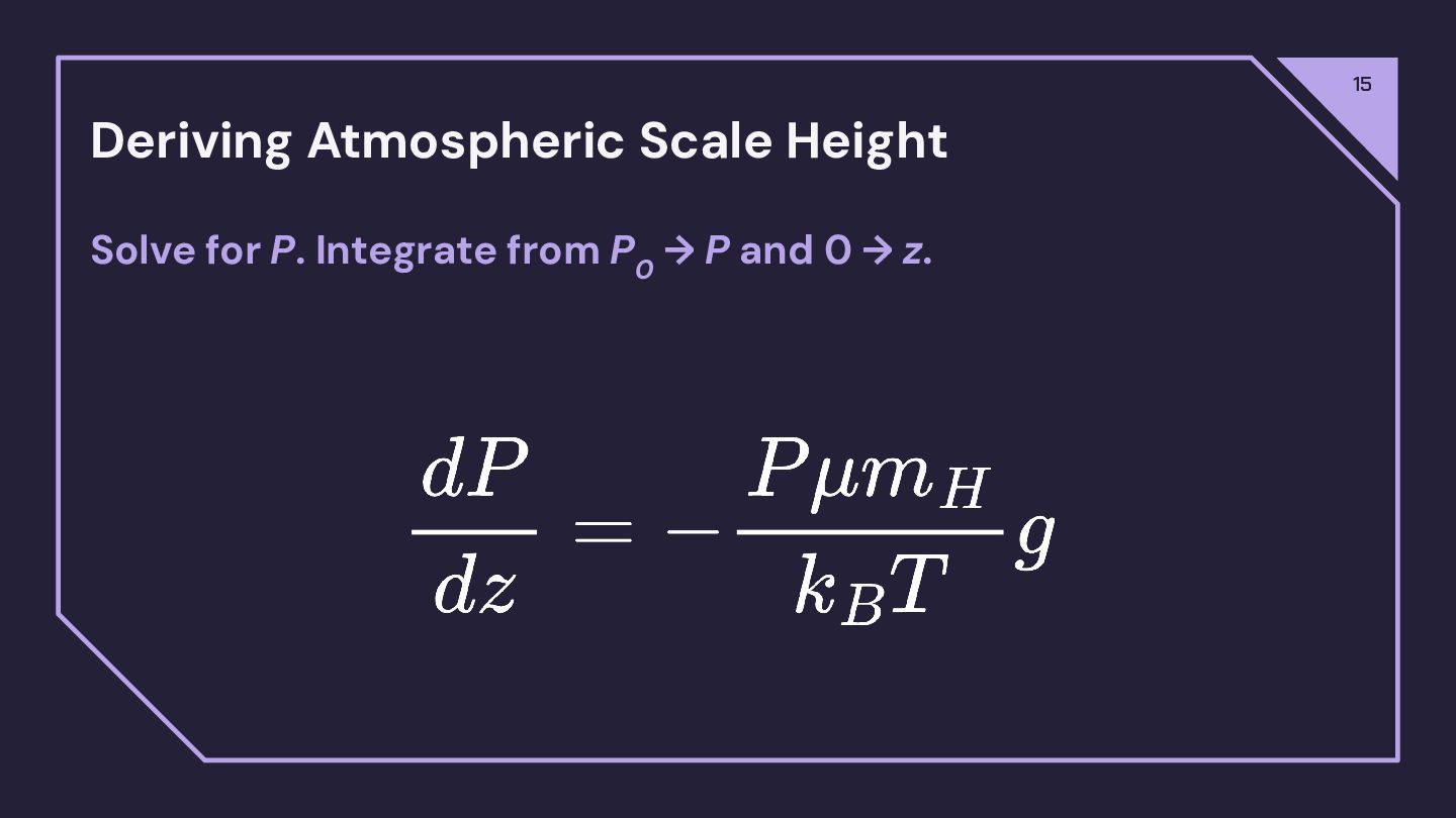
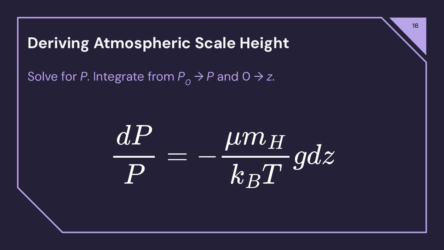
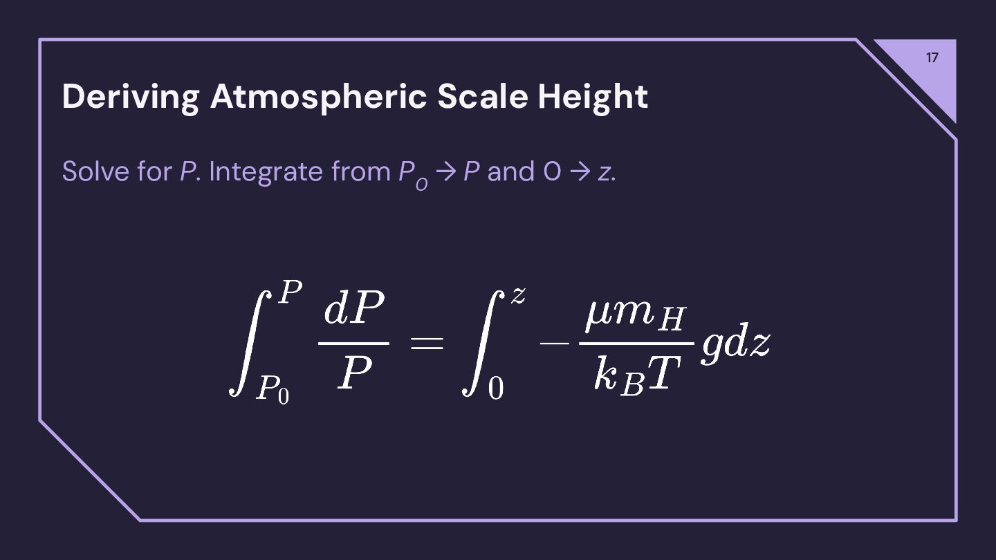
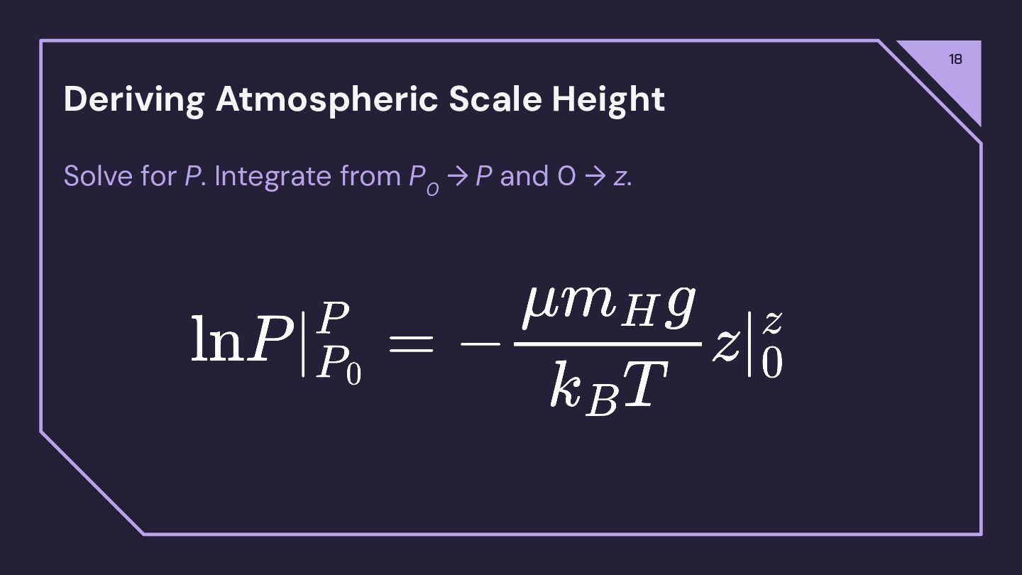
I will be sharing the slides I developed for a graduate level course on Exoplanets and Observational Astronomy. This is the fifth completed slide deck for this course. It covers topics on fundamentals of exoplanet atmospheres and atmospheric retrievals.

The atmospheric retrieval slides were adapted from Luis Welbanks.

Transcript

1. EXOPLANET ATMOSPHERES 1 Created by: Adina Feinstein
2. RELEVANT READINGS 2 Snellen (2025) Birkby (2018)
4. 4 TRANSMISSION
5. Orbital Phases - Transmission 5
6. Orbital Phases - Transmission 6 A planet’s atmosphere will be transparent at different wavelengths depending on what it is made of. The planet’s apparent radius (transit depth) is wavelength dependent.
7. Understanding the Components of a Transmission Spectrum 7 Carter et al. (2024)
8. Orbital Phases - Transmission 8 The strength of absorption features in a transmission spectrum will depend on the scale height of the atmosphere and the strength of the absorber. starlight
9. Orbital Phases - Transmission 9 The strength of absorption features in a transmission spectrum will depend on the scale height of the atmosphere and the strength of the absorption feature. starlight
10. 10 Deriving Atmospheric Scale Height The scale height is the increase in altitude for which the atmospheric pressure decreases by a factor of e.
11. 11 Deriving Atmospheric Scale Height Assume your atmosphere is in hydrostatic equilibrium. Gravity Pressure P = pressure z = height ρ = density g = gravitational acceleration
12. 12 Deriving Atmospheric Scale Height Assume the atmosphere is an ideal gas k B = Boltzmann constant T = Temperature μ = mean molecular weight m H = mass of hydrogen
13. 13 Deriving Atmospheric Scale Height Assume the atmosphere is an ideal gas k B = Boltzmann constant T = Temperature μ = mean molecular weight - average mass of a particle in m H = mass of hydrogen a mixture of gases [in amu]
14. 14 Deriving Atmospheric Scale Height Rearrange the ideal gas law to solve for ρ and plug into hydrostatic equilibrium.
15. 15 Deriving Atmospheric Scale Height Solve for P. Integrate from P 0 → P and 0 → z.
16. 16 Deriving Atmospheric Scale Height Solve for P. Integrate from P 0 → P and 0 → z.
17. 17 Deriving Atmospheric Scale Height Solve for P. Integrate from P 0 → P and 0 → z.
18. 18 Deriving Atmospheric Scale Height Solve for P. Integrate from P 0 → P and 0 → z.
19. 19 Deriving Atmospheric Scale Height Solve for P. Integrate from P 0 → P and 0 → z.
20. 20 Deriving Atmospheric Scale Height Solve for P. Integrate from P 0 → P and 0 → z.
21. 21 Deriving Atmospheric Scale Height Solve for P. Integrate from P 0 → P and 0 → z.
22. 22 Deriving Atmospheric Scale Height Solve for P. Integrate from P 0 → P and 0 → z.
23. 23 Deriving Atmospheric Scale Height For an H 2 -rich atmosphere (e.g., gas giants), μ = 2.3. Assuming a Jupiter-like planet with a temperature of 1500 K, calculate its scale height [in km].
24. 24 Deriving Atmospheric Scale Height For an Earth-like atmosphere, μ = 28. Assuming an Earth-like planet with a temperature of 300 K, calculate its scale height [in km].
25. Orbital Phases - Transmission 25 The strength of absorption features in a transmission spectrum will depend on the scale height of the atmosphere and the strength of the absorption feature.
26. Orbital Phases - Transmission 26 The scale height roughly tells you how “puffy” the atmosphere is. A larger scale height means the atmosphere extends farther above the opaque surface (or cloud deck). A small scale height means your atmosphere is more compressed and that the transmission features will be shallower (i.e. harder to detect).
27. Transmission - Who is better? 27 Hot Jupiter Cool Jupiter
28. Transmission - Who is better? 28 Hot Jupiter Cool Jupiter Hotter planets will have larger transmission features than cooler planets, given the H ∝T.
29. Transmission - Who is better? 29 Hot Jupiter Hot Neptune
30. Transmission - Who is better? 30 Planets with lower gravity will have larger scale heights, making large gas-giants, like Jupiter, easier to study. Hot Jupiter Hot Neptune
31. Transmission - Who is better? 31 A Venus-like planet An Earth-like planet
32. Transmission - Who is better? 32 A Venus-like planet An Earth-like planet Venus has a CO 2 dominated atmosphere (μ~44), whereas Earth has an O 2 /N 2 dominated atmosphere (μ~30). Planets with lower mean molecular weights will have larger features.
33. Scale Height - Realities 33 The scale height determines how many H’s worth of atmosphere you probe in transmission. On average, we probe ~3+ scale heights in puffy atmospheres (gas-giants). When deciding on what targets to observe, note that you will get the most signal from a target where you can observe the most Hs. Kempton et al. (2018)
34. How do we know what we’re actually seeing 34 The strength and shape of spectral features are governed by the wavelength-dependent cross-sections of specific molecules and the amount of absorbing material along the line of sight. Knowing this allows us to determine what is in a planet’s atmosphere.
35. Key Concepts 35 Opacity 𝛋(λ) - A measure of how much light is absorbed or scattered at a given wavelength [cm2/g].
36. Opacity 36 The opacity of an atmosphere will depend on:
37. Opacity 37 The opacity of an atmosphere will depend on: • The composition of the atmosphere (i.e. what molecules are present).
38. Opacity 38 The opacity of an atmosphere will depend on: • The composition of the atmosphere (i.e. what molecules are present). • The wavelength you observe at.
39. Opacity 39 The opacity of an atmosphere will depend on: • The composition of the atmosphere (i.e. what molecules are present). • The wavelength you observe at. • The temperature of the atmosphere.
40. Opacity 40 The opacity of an atmosphere will depend on: • The composition of the atmosphere (i.e. what molecules are present). • The wavelength you observe at. • The temperature of the atmosphere. • The pressure of the atmosphere (affects line broadening).
41. Opacity 41 Optical depth τ(λ) - the total opacity integrated along a path. Most features arise at τ(λ) ~ 1.
42. Connection to Transmission 42 At wavelengths where the opacity is high, the atmosphere becomes opaque higher up. This will result in a larger effective radius of the planet (i.e. a deeper transit).
43. Connection to Transmission 43 At wavelengths where the opacity is low, the atmosphere becomes opaque lower down. This will result in a smaller effective radius of the planet (i.e. a shallower transit).
44. Key Concepts 44 Opacity 𝛋(λ) - A measure of how much light is absorbed or scattered at a given wavelength [cm2/g]. Cross-section σ(λ) - The effective area an individual molecule presents to incoming light at a particular wavelength [cm2/molecule].
45. Cross-Sections 45 Different molecules absorb light at specific wavelengths, leading to distinct absorption features. Carter et al. (2024)
46. Cross-Sections 46 Good numbers to keep in mind (in microns): H 2 O - 0.9, 1.1, 1.4, 1.9, 2.7 CH 4 - 3.3 CO 2 - 4.3 Na - 0.589 Carter et al. (2024)
47. Side bar: Measuring Absorption Cross-Sections 47 The cross-sectional models we use to fit our transmission spectra must come from somewhere. Usually these models are a combination of laboratory and theoretical cross-sections. Why do we need both?
48. Side bar: Measuring Absorption Cross-Sections 48 Laboratory-measured cross-sections are limited. Every time a cross-section in measured, you have to assume a given temperature and pressure in your experiment.
49. Side bar: Measuring Absorption Cross-Sections 49 Examples of different lab techniques to measure cross-sections: Laser absorption spectrometry. Shine a laser through a concentration of species in the gas phase
50. Side bar: Measuring Absorption Cross-Sections 50 Examples of different lab techniques to measure cross-sections: Cavity ring-down spectroscopy (CRDS). Shine a laser into an optical cavity, which is bound by two highly reflective mirrors. When the laser is in resonance, intensity increases due to constructive interference. The laser is then turned off and you measure the decay in light intensity.
51. Side bar: Measuring Absorption Cross-Sections 51 Examples of different lab techniques to measure cross-sections: Cavity ring-down spectroscopy (CRDS). This method is (a) not sensitive to fluctuations in laser intensity, since you are measuring the decay and (b) very sensitive due to its long pathlength.
52. Side bar: Measuring Absorption Cross-Sections 52 Available cross-section libraries. • HITRAN - based on laboratory experiments. Good for Earth-like temperatures • HITEMP - higher temperature version of HITRAN • ExoMol - covers a range of temperatures, but specifically focuses on hot astrophysical environments Tennyson et al. (2016); Chubb et al. (2021); Gharib-Nezhad et al. (2021)
53. Key Concepts 53 Opacity 𝛋(λ) - A measure of how much light is absorbed or scattered at a given wavelength [cm2/g]. Cross-section σ(λ) - The effective area an individual molecule presents to incoming light at a particular wavelength [cm2/molecule]. Number density n - The number of molecules per unit volume [cm-3].
54. Aerosols, Clouds, and Hazes 54 Carter et al. (2024)
55. Clouds and Scattering 55 starlight
56. Clouds and Scattering 56 starlight
57. Clouds and Scattering 57 starlight
58. Aerosols, Clouds, and Hazes 58 Aerosols are particles suspended in a gas and includes clouds and hazes. Aerosols is the most generalized terminology.
59. Aerosols, Clouds, and Hazes 59 Aerosols are particles suspended in a gas and includes clouds and hazes. Aerosols is the most generalized terminology. A cloud - a visible mass of liquid and/or solid particles suspended in an atmosphere that form from the condensation of atmospheric gases. Hörst (2016)
60. Aerosols, Clouds, and Hazes 60 Aerosols are particles suspended in a gas and includes clouds and hazes. Aerosols is the most generalized terminology. A cloud - a visible mass of liquid and/or solid particles suspended in an atmosphere that form from the condensation of atmospheric gases. A haze - particles produced from chemistry in the atmosphere that results in the formation of involatile solids. Hazes do not go through cycles of evaporation and condensation. Hörst (2016)
61. Aerosols, Clouds, and Hazes (and dust) 61 Dust - solid particles that are suspended in the atmosphere that do not originate in the atmosphere. This is predominantly relevant for solar system bodies. Hörst (2016)
62. Why does it matter? 62 Hörst (2016)
63. Example: Titan 63 The formation of Titan's haze
64. Example: Titan 64 The formation of Titan's haze; Equatorial clouds on Titan
65. The role of aerosols 65 The presence of aerosols can dramatically change the structure of any given transmission spectrum. We know that the presence of a “cloud deck” will set the minimum measured transit depth of a planet.
66. The role of aerosols 66 The presence of aerosols can completely mute all transmission features. Kreidberg et al. (2014)
67. The role of aerosols 67 The presence of aerosols can induce a slope in the transmission spectrum due to scattering. Sing et al. (2015)
68. The role of aerosols 68 No two cloud-scattering slopes necessarily look the same. Sing et al. (2016)
69. Scattering Treatments 69 Rayleigh Scattering - The scattering of light off of the molecules in the atmosphere. Rayleigh scattering has a λ-4 dependence. Signature - blue slope Pont et al. (2013)
70. Scattering Treatments 70 Mie Scattering - The scattering of light off of larger atmospheric particles and has a ∝ λ dependence Signature - muted spectral features (no λ dependence) Schlawin et al. (2024)
71. Problems with Aerosols 71 The presence of aerosols (regardless of treatment) can cause many different degeneracies when trying to model exoplanet atmospheres. In a lot of ways, clouds/hazes will feel like a “band-aid” solution to weird features observed in transmission spectra.
72. 72 RETRIEVALS Adapted from Luis Welbanks
73. What is a retrievals? 73 A retrieval is a procedure to infer the atmospheric properties of an exoplanet from a set of observations. The inferred properties can include: chemical composition, vertical temperature structure, the presence of clouds/hazes, etc. Retrievals run a large ensemble of models to explore the parameter space that can best explain a set of observations.
74. 74 Retrieval Observed spectrum Model fit Chemical composition Parameter estimates
75. Why do we need retrievals? 75 Atmospheric models can be degenerate across multiple different parameters (e.g., high mean-molecular weight atmosphere versus clouds). By sampling the parameter space effectively, we can statistically quantify a “best-fit” model with “best-fit” properties. Data from Deming et al. 2013, Sing et al. 2016 Models Welbanks & Madhusudhan 2019
76. How do retrievals work? 76 Data from Deming et al. 2013, Sing et al. 2016
77. How do retrievals work? 77 Data from Deming et al. 2013, Sing et al. 2016
78. How do retrievals work? 78 Data from Deming et al. 2013, Sing et al. 2016
79. How do retrievals work? 79 Data from Deming et al. 2013, Sing et al. 2016
80. How do retrievals work? 80 Data from Deming et al. 2013, Sing et al. 2016
81. How do retrievals work? 81 Data from Deming et al. 2013, Sing et al. 2016
82. How do retrievals work? 82 Data from Deming et al. 2013, Sing et al. 2016
83. How do retrievals work? 83 Data from Deming et al. 2013, Sing et al. 2016
84. How do retrievals work? 84 Data from Deming et al. 2013, Sing et al. 2016
85. Deriving planetary parameters 85 Once you properly sample the parameter space for each property you are trying to fit, the resulting distribution will tell you the best-fit properties.
86. Deriving planetary parameters 86 Once you properly sample the parameter space for each property you are trying to fit, the resulting distribution will tell you the best-fit properties. Et voila! A corner plot.
87. What do we want from our retrieval? 87 Confidence intervals for the retrieved model. How do we get it: A family of models, with statistical meaning, that can explain the data. Data from Deming et al. 2013, Sing et al. 2016 Models Welbanks & Madhusudhan 2019
88. What do we want from our retrieval? 88 Inferences of other physical properties (e.g., vertical temperature structure) Data from Deming et al. 2013, Sing et al. 2016 Models Welbanks & Madhusudhan 2019
89. What do we want from our retrieval? 89 Statistical estimates of the model parameters Data from Deming et al. 2013, Sing et al. 2016 Models Welbanks & Madhusudhan 2019
90. What goes into an atmospheric retrieval? 90 Madhusudhan (2018)
91. What goes into an atmospheric retrieval? 91 Madhusudhan (2018)
92. The dirty details behind the black box 92 • Your favorite radiative transfer treatment
93. Radiative transfer assumptions 93 An atmospheric retrieval performance depends on the model’s efficiency to calculate radiative transfer in the planet’s atmosphere. A retrieval will run full radiative transfer models thousands to millions of times.
94. Radiative transfer assumptions 94 In an ideal world, we can run fully self-consistent 3D atmospheric models. In reality, “ain’t nobody got time for that.” Time per model Time per retrieval (106 models) ~10 ms ~2.7 hours ~50 ms ~13.5 hours ~ 0.5 days ~100 ms ~27.8 hours ~ 1.1 days ~1 s ~277.8 hours ~ 11.5 days ~1 min ~694 days ~ 2 years ~1 hour ~114 years ~1 day ~2740 years ~1 week ~20 millennia ~1 month ~Time since the Ice Age
95. Radiative transfer assumptions 95 Semi-analytic Models Numerical Models
96. Radiative transfer assumptions 96 Semi-analytic Models Pros: • Fast to compute Numerical Models
97. Radiative transfer assumptions 97 Semi-analytic Models Pros: • Fast to compute Cons: • Isothermal + isobaric assumptions • Fixed gravity • Limited number of absorbers Numerical Models
98. Radiative transfer assumptions 98 Semi-analytic Models Pros: • Fast to compute Cons: • Isothermal + isobaric assumptions • Fixed gravity • Limited number of absorbers Numerical Models Pros: • Does not rely on isothermal, isobaric, gravity assumptions • Can include multiple absorbers
99. Radiative transfer assumptions 99 Semi-analytic Models Pros: • Fast to compute Cons: • Isothermal + isobaric assumptions • Fixed gravity • Limited number of absorbers Numerical Models Pros: • Does not rely on isothermal, isobaric, gravity assumptions • Can include multiple absorbers Cons: • Can be comparatively slower to compute
100. Radiative transfer assumptions 100 Semi-analytic Models Numerical Models YOUR MODEL ASSUMPTIONS WILL AFFECT YOUR INFERRED ATMOSPHERIC PROPERTIES.
101. The dirty details behind the black box 101 • Your favorite radiative transfer treatment • Some relationship between atmospheric pressure and temperature
102. Pressure-temperature (PT) profiles 102 To ease model computation, we want to use a parametric treatment that allows us to capture the vertical temperature structure of the atmosphere. A robust treatment should be able to capture the physical behavior we expect (e.g., thermal inversions, the profile of non-irradiated objects, etc.). Gandhi & Madhusudhan (2018)
103. Pressure-temperature (PT) profiles 103 Effective P-T parameterizations with a minimal number of free parameters are critical! This is especially important for emission spectroscopy, where the spectrum is sensitive to temperature gradients. Examples: Madhusudhan & Seager 2009, Guillot 2010, Line et al. 2013, Burningham et al. 2017, Blecic et al. 2017, Piette & Madhusudhan 2021. Madhusudhan & Seager (2009)
104. Example parameterization: Madhusudhan & Seager (2009) 104 • Motivated by the vertical temperature structure of irradiated atmospheres (self-consistent models of hot Jupiters and solar system planets) • Includes a mesosphere, stratosphere (where spectral features arise from) and a deep isothermal layer Madhusudhan & Seager (2009)
105. Example parameterization: Guillot (2010) 105 • Physically motivated prescription • Two-stream approximation - only includes two wavelength channels (thermal and visible) • The model was extended by Line (2013) to include a second visible opacity to allow for thermal inversions. • Included in PLATON and petitRADTRANS (open-source retrievals) Guillot (2010)
106. The dirty details behind the black box 106 • Your favorite radiative transfer treatment • Some relationship between atmospheric pressure and temperature • Chemistry treatment - equilibrium or disequilibrium?
107. Chemical assumptions 107 Free Retrieval Chemically consistent (equilibrium) Self-consistent More assumptions More free parameters
108. Chemical assumptions - Free retrievals 108 • Chemical composition is represented by volume mixing ratios (VMR) and are fit as free parameters. • Chemical composition is assumed to be uniform in the atmospheric region probed by the observations. • Less time consuming since it is not restricted by chemical equilibrium.
109. Chemical assumptions - Free retrievals 109 ⚠ WARNING ⚠ • Free retrievals have a risk of “overfitting” the data. • Sensitive to adding unexpected chemical species. • The solution may be unphysical - need to use your judgement
110. Chemical assumptions - Chemical Equilibrium 110 • Given a set of parameters (e.g., metallicity, C/O), the abundances are computed using an equilibrium chemistry prescriptions. • Abundances determined by minimizing the Gibbs free energy of the system for a given temperature, pressure, and elemental abundances. • The equilibrium computation can vary in complexity.
111. Chemical assumptions - Chemical Equilibrium 111 ⚠ WARNING ⚠ • The spectral fit can be worse than what is obtained via a free retrieval because of additional restrictions. • Disequilibrium conditions will not be captured by these models.
112. Chemical assumptions - Example differences 112 Chemical equilibrium retrieval suggests super-solar oxygen abundance log 10 (O/O ⊙ ) = 1.21 ± 0.16 log 10 (C/C ⊙ ) = 1.41 ± 0.18 log 10 (Na/Na ⊙ ) = 0.94 ± 0.51 Spake et al. (2021)
113. Chemical assumptions - Example differences 113 Free retrieval suggests sub-solar oxygen abundance from H 2 O VMR log 10 (H 2 O) = -4.16 ± 0.19 VMR log 10 (CO 2 ) = -5.52 ± 0.43 VMR log 10 (Na) = -6.99 ± 0.39 Spake et al. (2021)
114. Chemical assumptions - Example differences 114 Even on the same spectroscopic observations, different modeling strategies can result in different inferences. Spake et al. (2021)
115. The dirty details behind the black box 115 • Your favorite radiative transfer treatment • Some relationship between atmospheric pressure and temperature • Chemistry treatment - equilibrium or disequilibrium? • Composition and cloud parameterization
116. Composition 116
117. Composition 117 You can retrieve your cross sections from ExoMol, HITRAN/HITEMP, or your favorite laboratory or theoretical effort. The radiative transfer is calculated on a fine grid to resolve individual chemical lines. Don’t forget to consider: pressure dependence, temperature dependence, and sources of continuum opacity.
118. Composition 118 Many codes assume the atmosphere will be H 2 -rich. Alternatively, you can “hardcode” a non H 2 -rich composition or you can aim to agnostically retrieve the bulk composition of the atmosphere. Be aware of the bulk composition assumptions and the limitations of any model!
119. Cloud parameterization 119 We want to obtain a robust inference on our atmospheric composition and vertical structure without biasing our results by the impact of clouds and/or hazes.
120. Cloud parameterization 120 We want to obtain a robust inference on our atmospheric composition and vertical structure without biasing our results by the impact of clouds and/or hazes. Clouds - condensates, large particles, flattens a spectrum. Barstow (2021)
121. Cloud parameterization 121 We want to obtain a robust inference on our atmospheric composition and vertical structure without biasing our results by the impact of clouds and/or hazes. Hazes - photochemistry, small particles, introduces a scattering slope to the spectrum. Barstow (2021)
122. The dirty details behind the black box 122 • Your favorite radiative transfer treatment • Some relationship between atmospheric pressure and temperature • Chemistry treatment - equilibrium or disequilibrium? • Composition and cloud parameterization • Others: ◦ Stellar effects (spots, flares, granulation) ◦ Deviations from plane-parallel radiative transfer equation
123. 123 EMISSION
124. Orbital Phases - Emission 124
125. Emission Spectroscopy 125 An emission spectrum probes the brightness temperature in the atmosphere as a function of wavelength. Emission spectra provide key constraints on temperature profiles of giant exoplanets or albedo properties for small exoplanets.
126. Emission Spectroscopy 126 Observable: the planet-to-star flux ratio (F p /F S ) If reflected light from the star dominates, • A G is the geometric albedo • R p is the radius of the planet • a is the orbital separation
127. Geometric albedo 127 The geometric albedo is the ratio of the actual brightness of an object to that of an idealized flat, fully reflecting disk with the same cross-section. Whereas the bond albedo is the fraction of power in the EM radiation spectrum that is scattered back into space. Planet A G Mercury 0.142 Venus 0.689 Earth 0.434 Mars 0.17 Jupiter 0.538 Saturn 0.499 Uranus 0.488 Neptune 0.442
128. 128 How atmospheres affect the measured brightness temperature https://science.nasa.gov/mission/webb/science-overview/science-explainers/can-rocky-worlds-orbiting-red-dwarf-stars-maintain-atmospheres/
129. 129 Kreidberg & Stevenson (2025) Rocky planet dayside brightness temperatures with JWST
130. Emission Spectroscopy 130 If thermal emission from the planet dominates, • A G is the geometric albedo • R p is the radius of the planet • R ★ is the radius of the star • B λ (T) is the blackbody function of the planet and star at temperatures, T p and T ★
131. Advantages 131 The advantage of emission spectroscopy is that you are probing the full dayside of the planet, rather than just the limbs from transmission.
132. Example gas giant emission spectrum 132 Wiser et al. (2025)
133. 133 Wiser et al. (2025)
134. 134 PHASE CURVES
135. Orbital Phases - Phase Curve 135
136. Orbital Phases - Phase Curve 136
137. 137 Orbital Phases - Phase Curve The curvature we see from a full orbital phase curve is determined by the contribution of reflected or thermal light from the planet.
138. 138 The first full phase curve - HD 189733b F p /F ★ = 0.1466 % at 3.6μm F p /F ★ = 0.1787 % at 4.5μm Knutson et al. (2019)
139. 139 Deriving the dayside temperature of HD 189733b Knutson et al. (2019) R p /R ★ = 0.155 T eff = 5050 K F p /F ★ = 0.1466 % at 3.6μm F p /F ★ = 0.1787 % at 4.5μm Calculate T p .
140. 140 3D Global Circulation Models Atmospheric circulation models of hot Jupiters show: • A horizontal temperature contrast is maintained (contours). Showman & Guillot (2002)
141. 141 3D Global Circulation Models Atmospheric circulation models of different of hot Jupiters show: • An equatorial jet contains most of the kinetic energy and shows both eastward and westward branches. Showman & Guillot (2002)
142. 142 3D Global Circulation Models Atmospheric circulation models of different of hot Jupiters show: • Winds that develop away from the equator skirt parallel to the temperature contours. This is evidence that the Coriolis force is balanced by the pressure-gradient force. Showman & Guillot (2002)
143. First spectroscopic eclipse map - WASP-18b 143 Challener et al. (2025) Now, with JWST, we can observe a spectroscopic eclipse map. The maps reveal two thermally distinct regions of the planet’s atmosphere: a hotspot and a ring near the bayside limbs. More details on the mapping technique can be found in Mansfield et al. (2020).
144. First spectroscopic eclipse map - WASP-18b 144 Challener et al. (2025) Hotspot - shows the presence of water absorption, although it is weaker than the hemispheric average.
145. First spectroscopic eclipse map - WASP-18b 145 Challener et al. (2025) Hotspot - shows the presence of water absorption, although it is weaker than the hemispheric average. Ring - shows a colder temperature and no strong evidence of any absorbers.
146. ESA’s Atmospheric Remote-sensing Infrared Exoplanet Large-survey (ARIEL) Mission 146 Objective: Perform a chemical consensus of a large, diverse set of exoplanets. Instrument: 1.95 - 7.8 μm spectrograph at R ~ 100 (comparable to JWST NIRSpec/PRISM) Expected Launch: 2029
148. 148 HIGH-RESOLUTION SPECTROSCOPY
149. High resolution appearance of a planet as a function of phase 149 Snellen (2025) Yellow = stellar; black = telluric
150. The effects of decreasing spectral resolution 150 This is an example specifically for CO. R Blue = 30,000 R Red = 5,000 R green = 300 R black = 30 Birkby (2018)
151. High-resolution reduction 151 Here is an example of the stages of the telluric removal process using principal component analysis. Birkby (2018)
152. High-resolution reduction 152 A) The raw observed extracted stellar spectra Birkby (2018)
153. High-resolution reduction 153 B) The normalized spectra Birkby (2018)
154. High-resolution reduction 154 C) After removing the first principal component Birkby (2018)
155. High-resolution reduction 155 D) After removing optimal components Birkby (2018)
156. High-resolution reduction 156 E) The same as D but with a model water spectrum injected at stage A at 100× the nominal planet single strength Birkby (2018)
157. Cross-correlation technique 157 Snellen (2025) In order to detect a species at high resolution, we use a cross-correlation technique, which is model dependent.
158. Detection of H 2 O in HD 189733 b 158 Birkby (2018)
159. Overview of the elements detected in Ultra-Hot Jupiters 159 Snellen (2025)
160. Heatmap of atomic and molecular detections in ultra-hot Jupiters 160 Feinstein et al. (2025)
161. The presence of thermal inversions 161 There is a clear relationship between whether a planet has an inversion or not and the T eq of the planet. Snellen (2025)
162. 162 JWST BREAKDOWN
163. 163 NIRISS Single Object Slitless Spectrograph (SOSS): 0.6 - 2.8 micron
164. 164 NIRCam Spectroscopy
165. 165 NIRSpec Spectroscopy
166. 166 MIRI Photometry
167. 167 MIRI Low-Resolution Spectroscopy: 5-12 micron
168. 168 Excellent recent colloquium from Dr. Brett Morris - https://mediaspace.msu.edu/media/Physics+and+Astronomy+C olloquium+delivered+by+Dr.+Brett+Morris+%28STScI%29/1_mjtp utb2