I will be sharing the slides I developed for a graduate level course on Exoplanets and Observational Astronomy. This is the seventh and final completed slide deck for this course. It covers topics on microlensing. In theory, it should cover topics such as astrometry and microlensing as well, however class time did not allow for these topics to be covered.
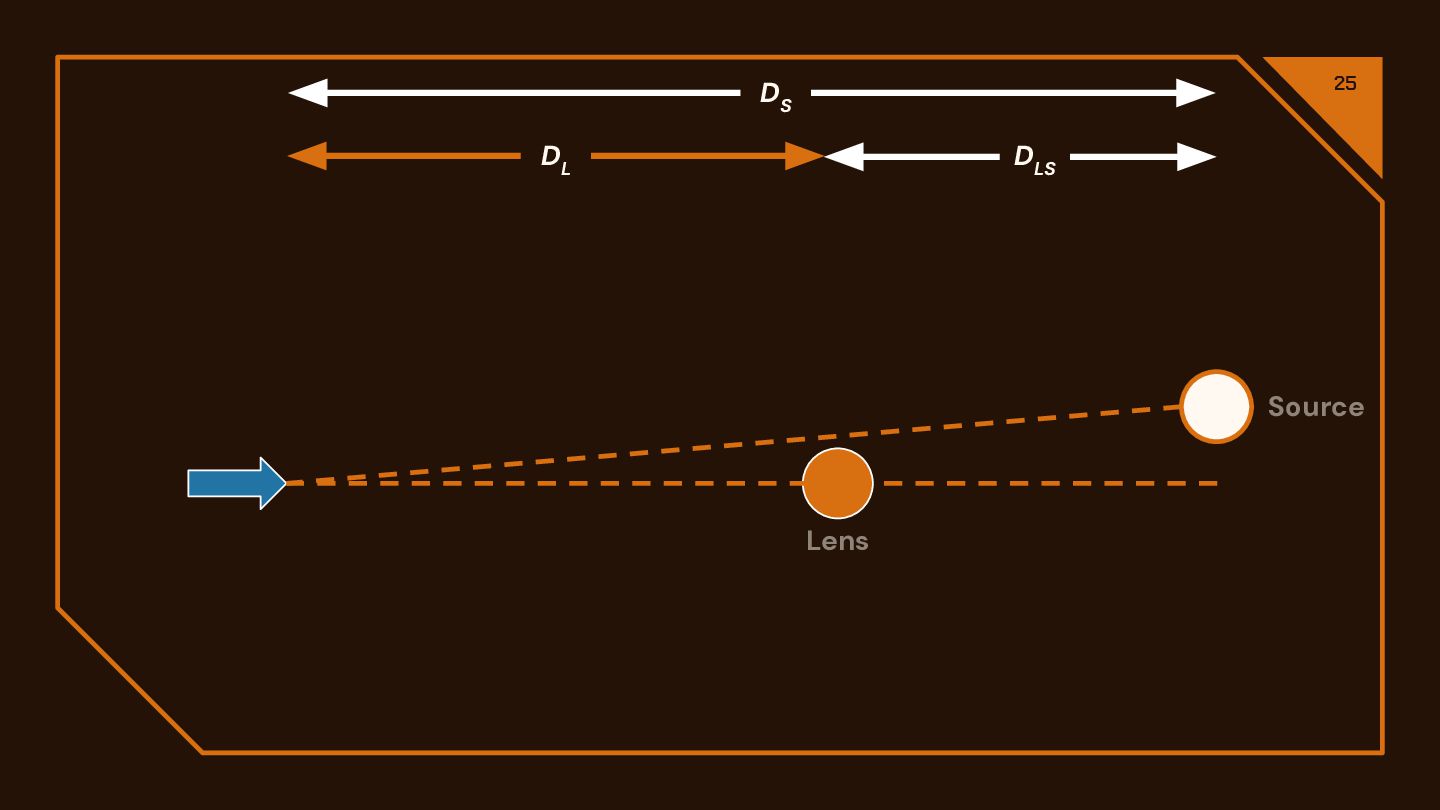
![26 Image 1 [-] Source Lens θ S θ I](https://files.speakerdeck.com/presentations/8d22023fb36a45748bfeb1f5c2936043/slide_25.jpg)
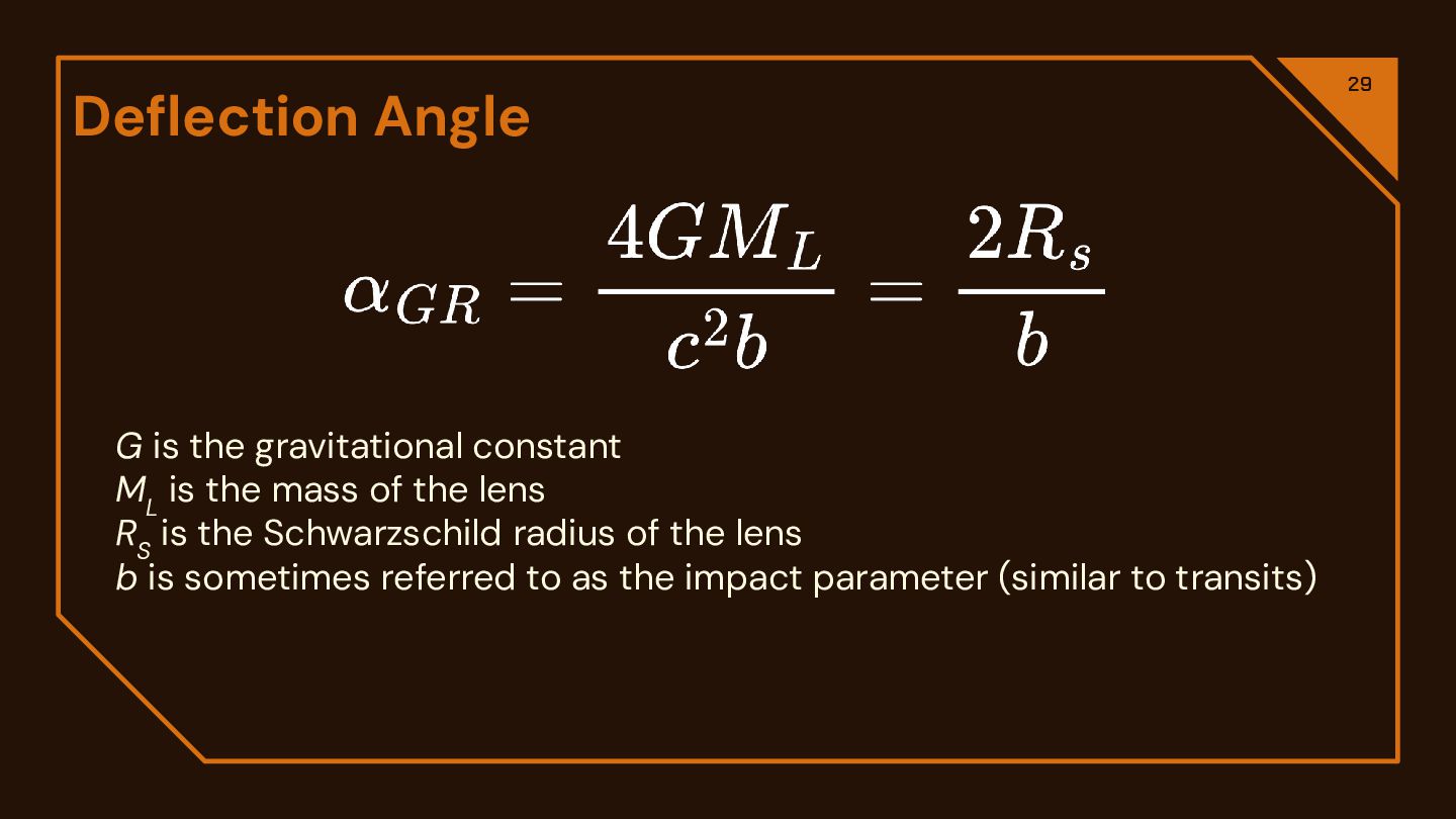
![27 Image 1 [-] Source Lens ɑ GR Image 1](https://files.speakerdeck.com/presentations/8d22023fb36a45748bfeb1f5c2936043/slide_26.jpg)
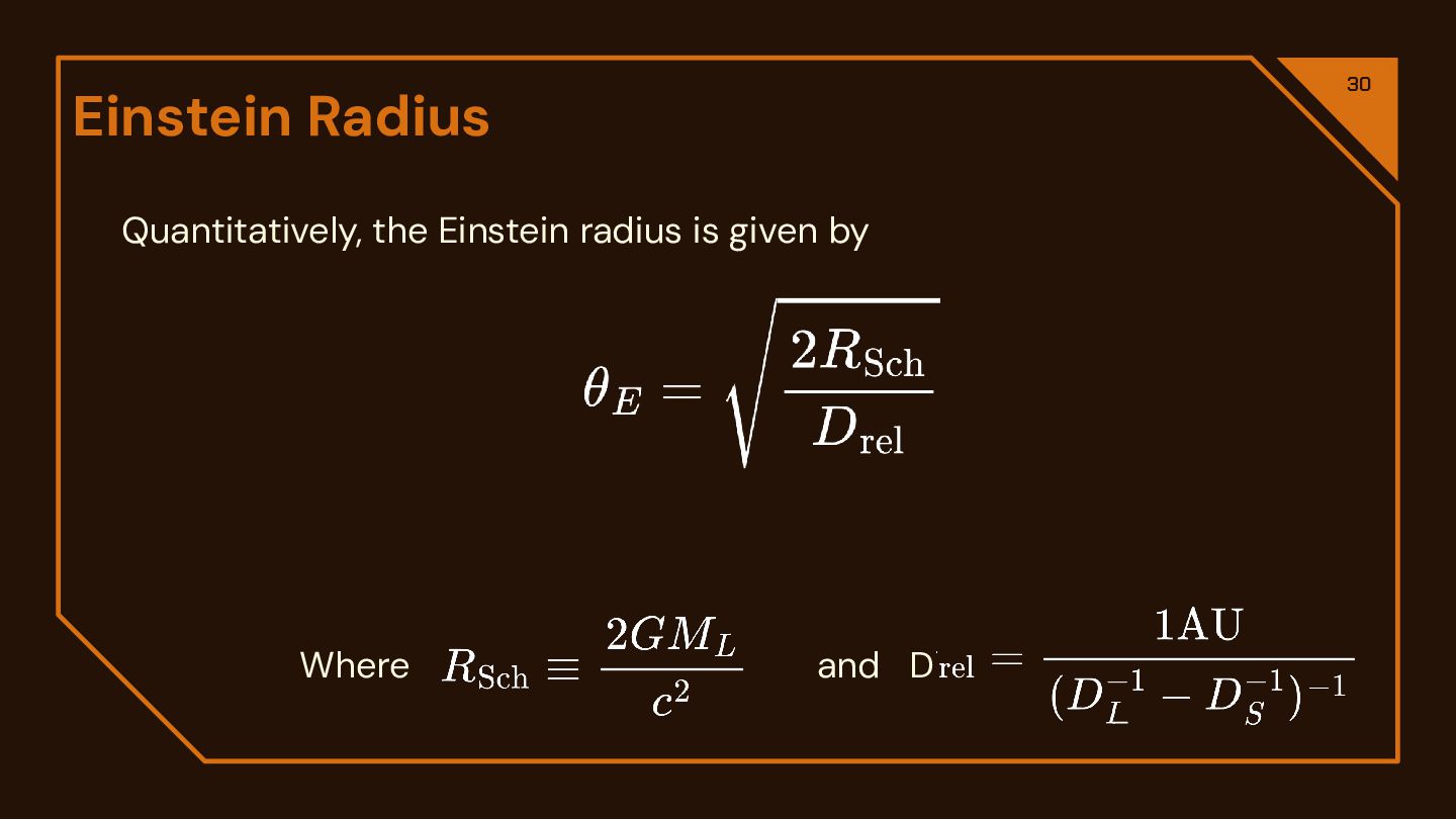
![28 Image 1 [+] Image 1 [-] Source Lens ɑ](https://files.speakerdeck.com/presentations/8d22023fb36a45748bfeb1f5c2936043/slide_27.jpg)