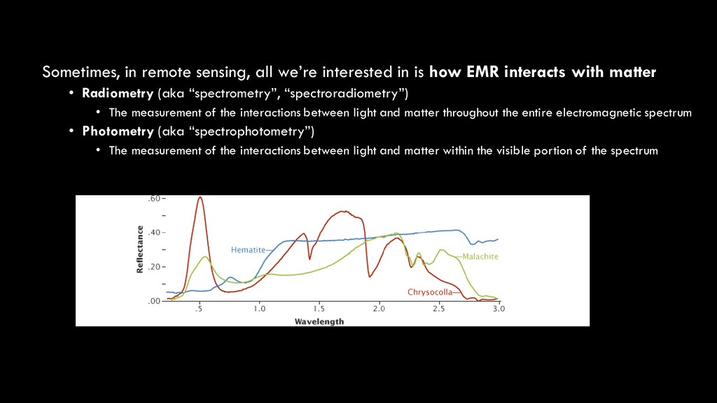
EMR interacts with matter • Radiometry (aka “spectrometry”, “spectroradiometry”) • The measurement of the interactions between light and matter throughout the entire electromagnetic spectrum • Photometry (aka “spectrophotometry”) • The measurement of the interactions between light and matter within the visible portion of the spectrum
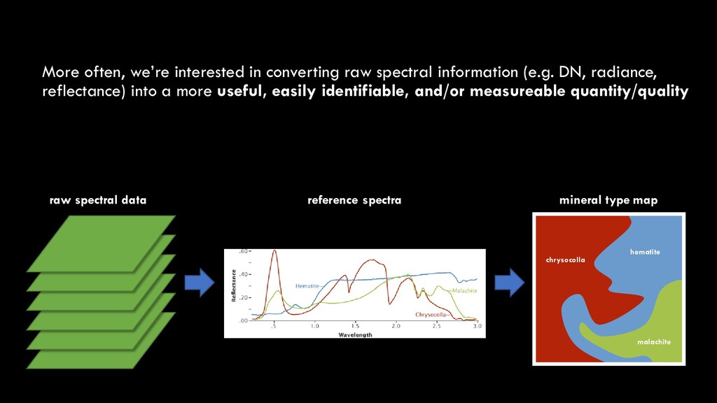
DN, radiance, reflectance) into a more useful, easily identifiable, and/or measureable quantity/quality raw spectral data reference spectra mineral type map chrysocolla malachite hematite
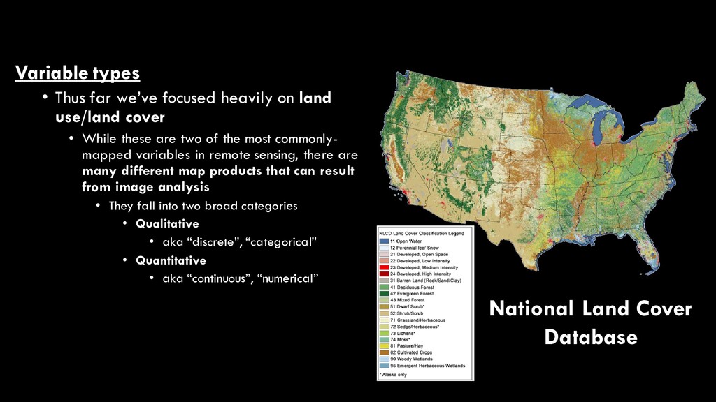
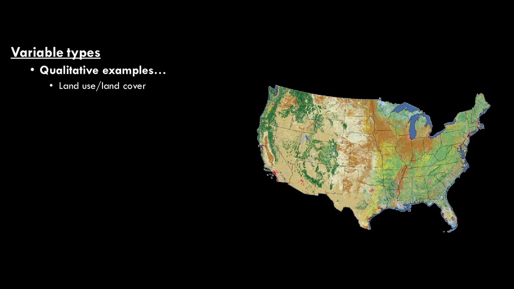
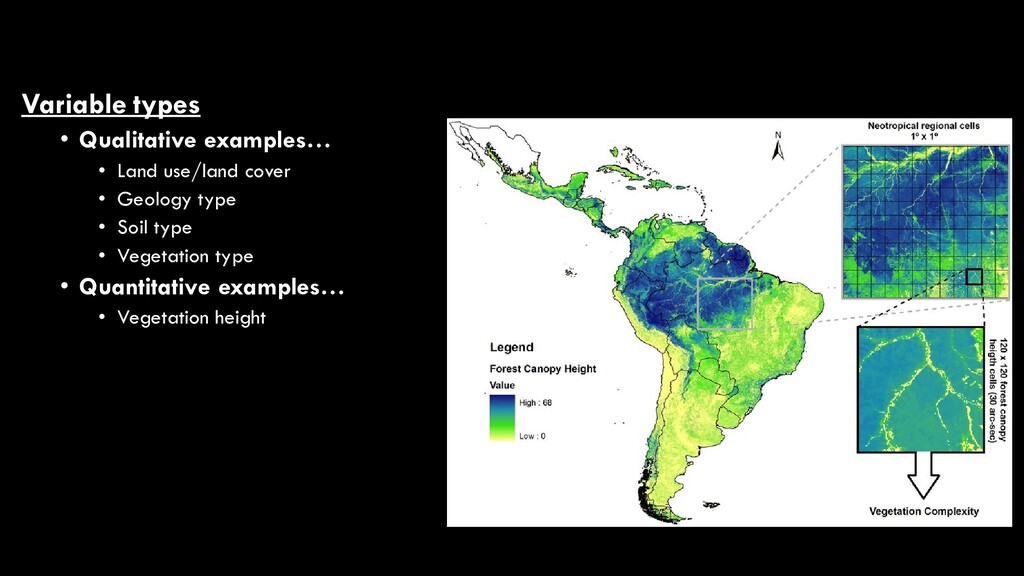
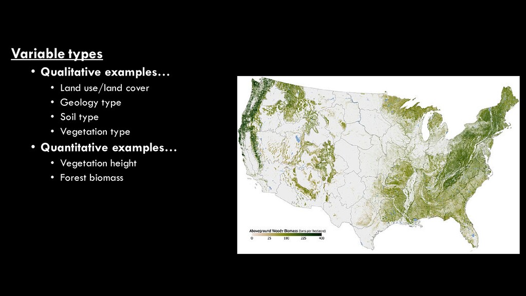
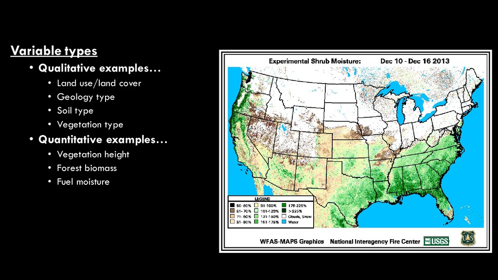
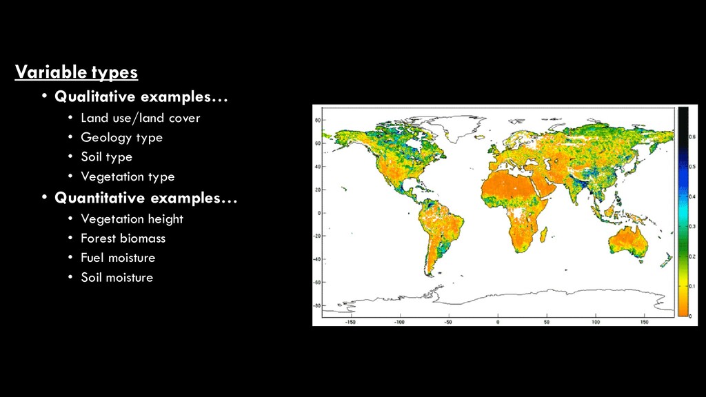
use/land cover • While these are two of the most commonly- mapped variables in remote sensing, there are many different map products that can result from image analysis • They fall into two broad categories • Qualitative • aka “discrete”, “categorical” • Quantitative • aka “continuous”, “numerical” National Land Cover Database
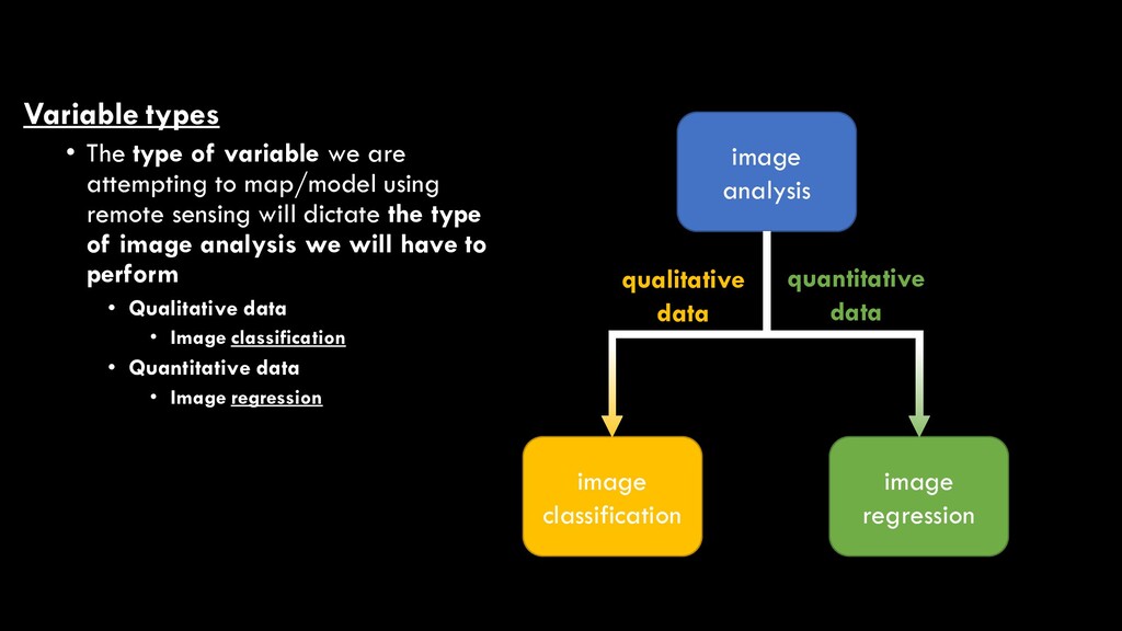
to map/model using remote sensing will dictate the type of image analysis we will have to perform • Qualitative data • Image classification • Quantitative data • Image regression image analysis image classification image regression qualitative data quantitative data
What is a statistical model? Not as complicated as it sounds, that’s what. • A mathematically-based, simplified approximation of reality • That approximation is often used to make predictions about some variable of interest
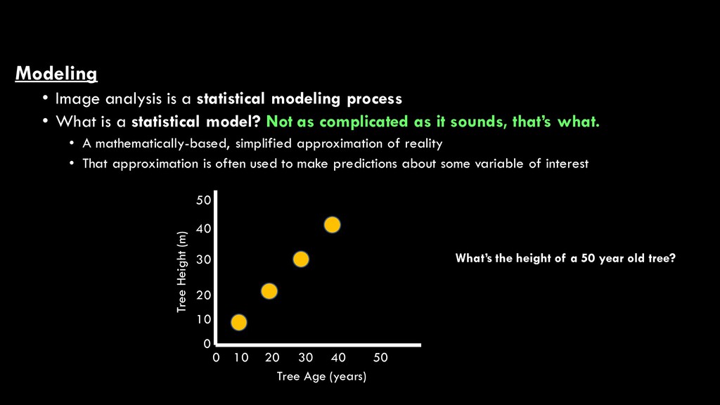
What is a statistical model? Not as complicated as it sounds, that’s what. • A mathematically-based, simplified approximation of reality • That approximation is often used to make predictions about some variable of interest Tree Height (m) Tree Age (years) 0 10 20 30 40 50 0 10 20 30 40 50 What’s the height of a 50 year old tree?
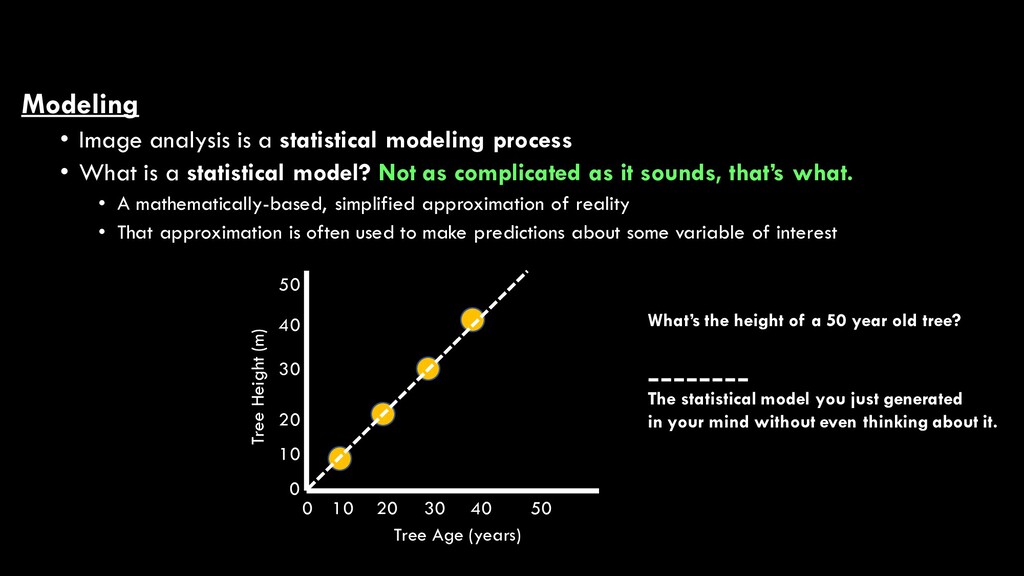
What is a statistical model? Not as complicated as it sounds, that’s what. • A mathematically-based, simplified approximation of reality • That approximation is often used to make predictions about some variable of interest Tree Height (m) Tree Age (years) 0 10 20 30 40 50 0 10 20 30 40 50 What’s the height of a 50 year old tree? The statistical model you just generated in your mind without even thinking about it.
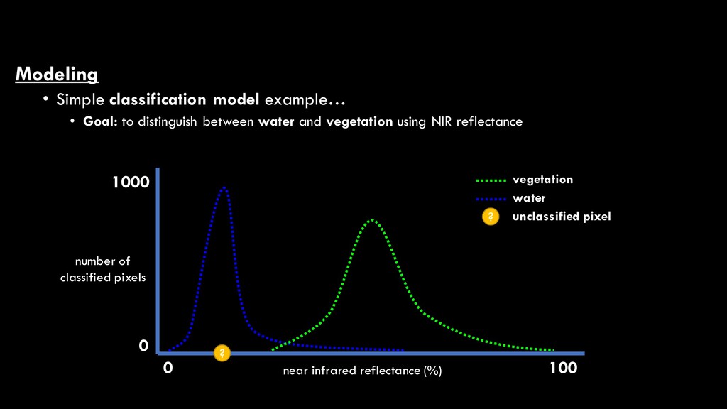
between water and vegetation using NIR reflectance near infrared reflectance (%) 0 100 0 1000 vegetation water ? ? unclassified pixel number of classified pixels
between water and vegetation using NIR reflectance near infrared reflectance (%) 0 100 0 1000 vegetation water ? ? unclassified pixel number of classified pixels
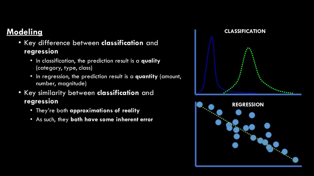
classification, the prediction result is a quality (category, type, class) • In regression, the prediction result is a quantity (amount, number, magnitude) • Key similarity between classification and regression • They’re both approximations of reality • As such, they both have some inherent error CLASSIFICATION REGRESSION
classification • Unsupervised image classification • Image data are grouped together into discrete classes according to spectral similarity alone, without the influence of reference data to dictate the grouping process • Supervised image classification • Image data are grouped together into discrete classes according to the degree to which spectral information in unsampled areas correspond with known spectral information derived from a set of reference data
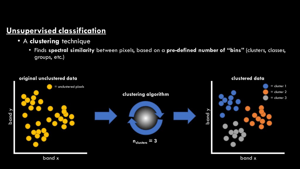
between pixels, based on a pre-defined number of “bins” (clusters, classes, groups, etc.) clustering algorithm nclusters = 3 band x band y original unclustered data = unclustered pixels band x band y clustered data = cluster 1 = cluster 2 = cluster 3
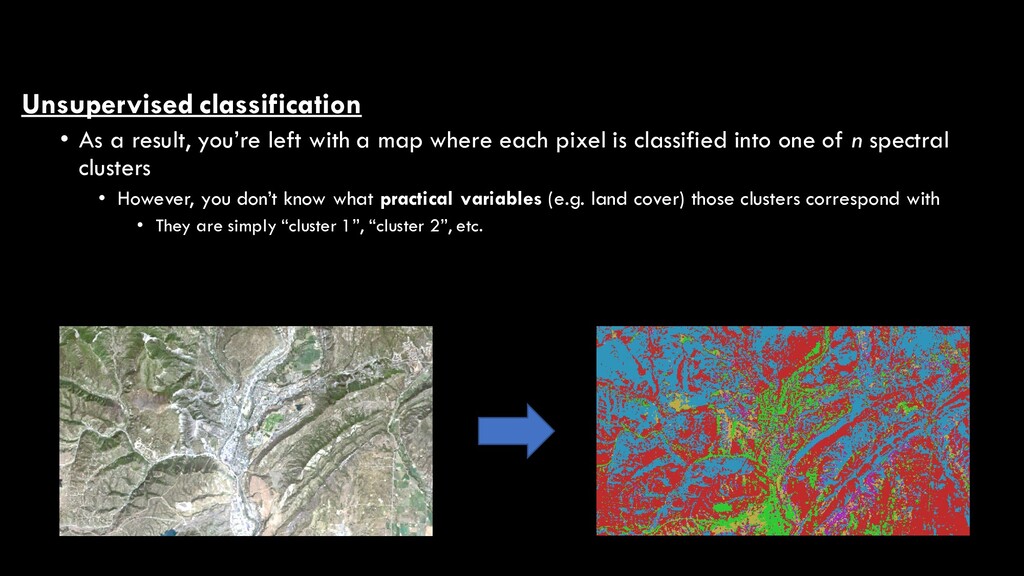
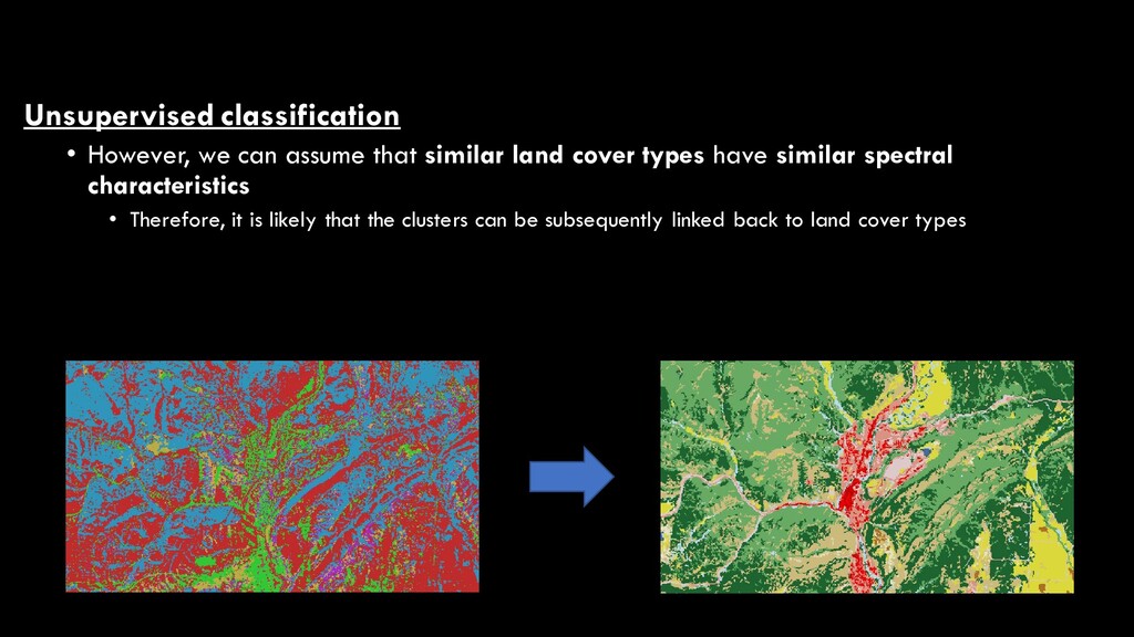
map where each pixel is classified into one of n spectral clusters • However, you don’t know what practical variables (e.g. land cover) those clusters correspond with • They are simply “cluster 1”, “cluster 2”, etc.
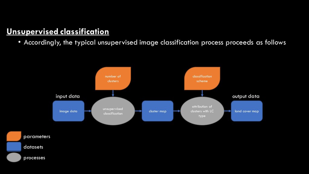
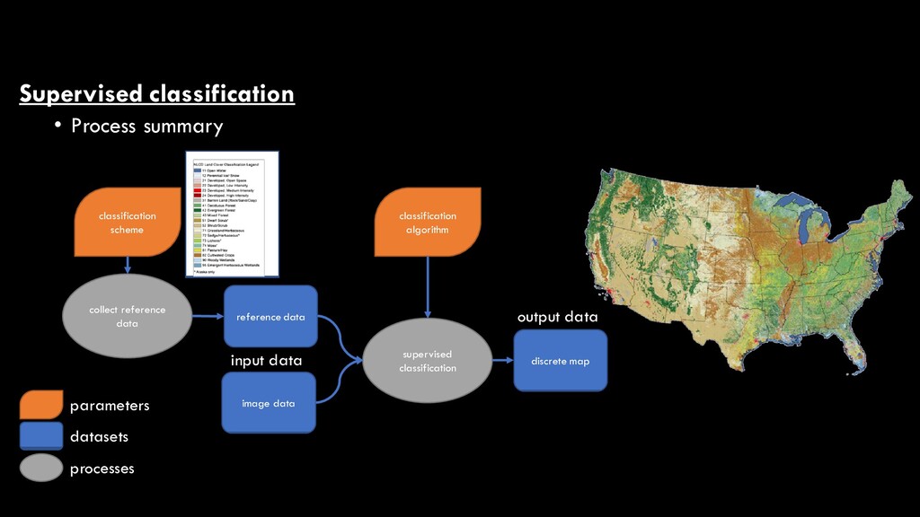
proceeds as follows image data unsupervised classification cluster map attribution of clusters with LC type land cover map number of clusters classification scheme input data output data parameters datasets processes
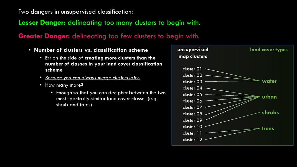
the side of creating more clusters than the number of classes in your land cover classification scheme • Because you can always merge clusters later. • How many more? • Enough so that you can decipher between the two most spectrally-similar land cover classes (e.g. shrub and trees) cluster 01 cluster 02 cluster 03 cluster 04 cluster 05 cluster 06 cluster 07 cluster 08 cluster 09 cluster 10 cluster 11 cluster 12 water urban shrubs trees unsupervised map clusters land cover types Greater Danger: delineating too few clusters to begin with. Lesser Danger: delineating too many clusters to begin with. Two dangers in unsupervised classification:
less-commonly used than supervised classification in remote sensing analyses • It’s a great data exploration/mining technique • It lets the data speak for themselves • It can help illuminate patterns/trends in your data that you might not have recognized otherwise • It’s great when you don’t have reference data
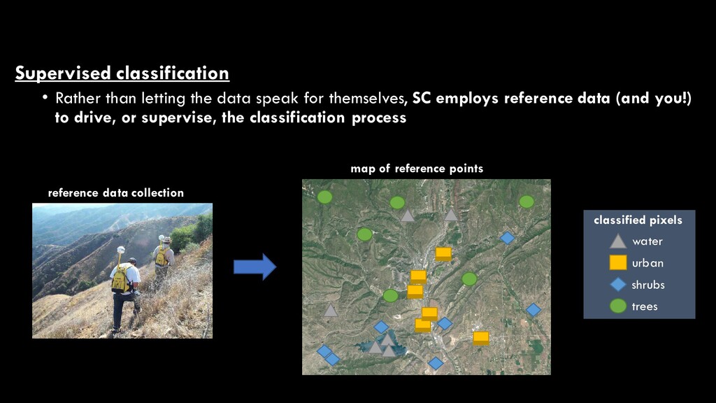
themselves, SC employs reference data (and you!) to drive, or supervise, the classification process reference data collection water urban shrubs trees classified pixels map of reference points
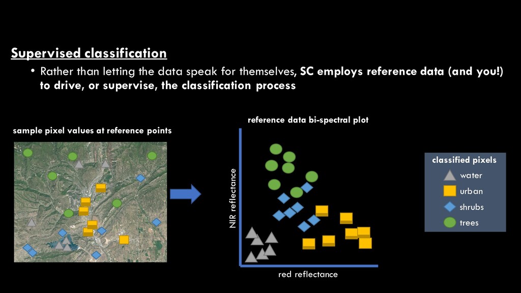
themselves, SC employs reference data (and you!) to drive, or supervise, the classification process red reflectance NIR reflectance reference data bi-spectral plot sample pixel values at reference points water urban shrubs trees classified pixels
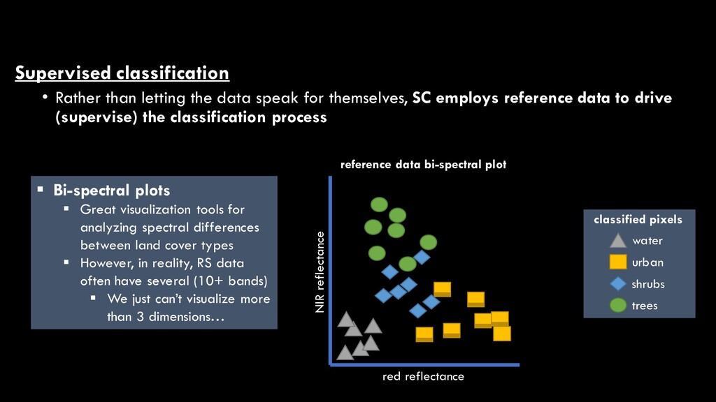
themselves, SC employs reference data to drive (supervise) the classification process red reflectance NIR reflectance reference data bi-spectral plot water urban shrubs trees classified pixels Bi-spectral plots Great visualization tools for analyzing spectral differences between land cover types However, in reality, RS data often have several (10+ bands) We just can’t visualize more than 3 dimensions…
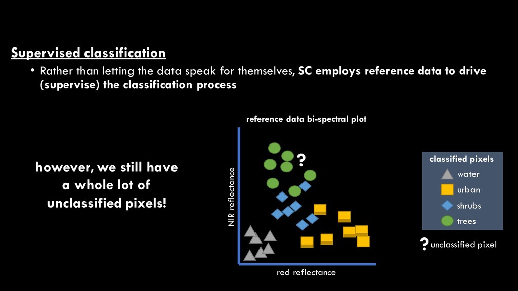
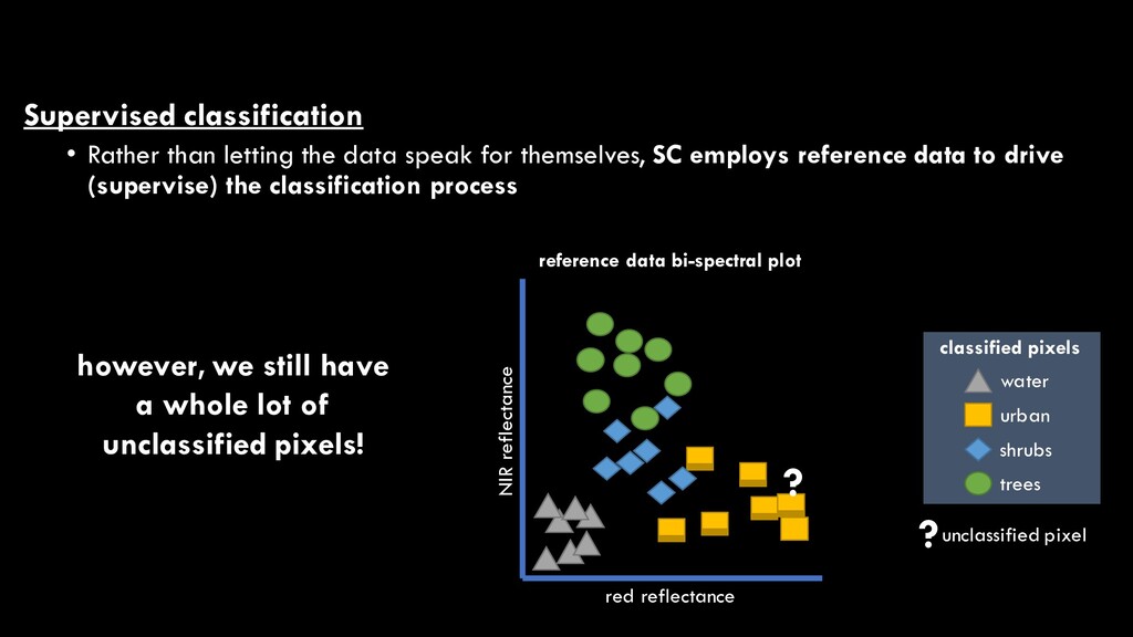
themselves, SC employs reference data to drive (supervise) the classification process however, we still have a whole lot of unclassified pixels! ?unclassified pixel red reflectance NIR reflectance reference data bi-spectral plot water urban shrubs trees classified pixels ?
themselves, SC employs reference data to drive (supervise) the classification process however, we still have a whole lot of unclassified pixels! ?unclassified pixel red reflectance NIR reflectance reference data bi-spectral plot water urban shrubs trees classified pixels ?
themselves, SC employs reference data to drive (supervise) the classification process however, we still have a whole lot of unclassified pixels! ?unclassified pixel red reflectance NIR reflectance reference data bi-spectral plot water urban shrubs trees classified pixels ?
themselves, SC employs reference data to drive (supervise) the classification process however, we still have a whole lot of unclassified pixels! ?unclassified pixel red reflectance NIR reflectance reference data bi-spectral plot water urban shrubs trees classified pixels ?
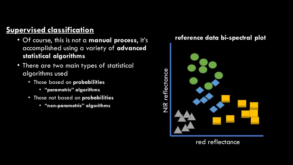
process, it’s accomplished using a variety of advanced statistical algorithms • There are two main types of statistical algorithms used • Those based on probabilities • “parametric” algorithms • Those not based on probabilities • “non-parametric” algorithms red reflectance NIR reflectance reference data bi-spectral plot
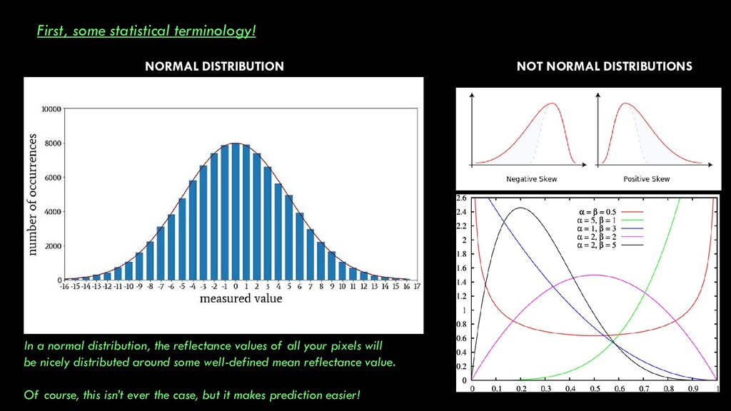
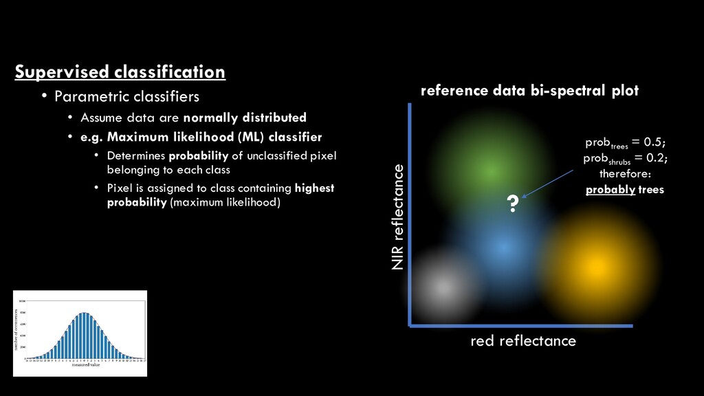
a normal distribution, the reflectance values of all your pixels will be nicely distributed around some well-defined mean reflectance value. Of course, this isn’t ever the case, but it makes prediction easier!
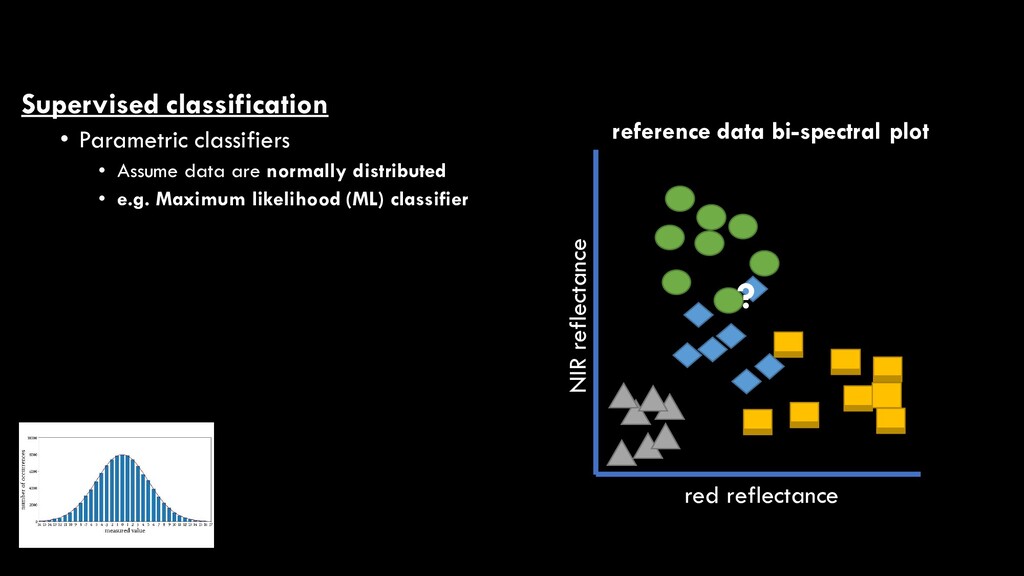
distributed • e.g. Maximum likelihood (ML) classifier • Determines probability of unclassified pixel belonging to each class • Pixel is assigned to class containing highest probability (maximum likelihood) red reflectance NIR reflectance reference data bi-spectral plot ? probtrees = 0.5; probshrubs = 0.2; therefore: probably trees
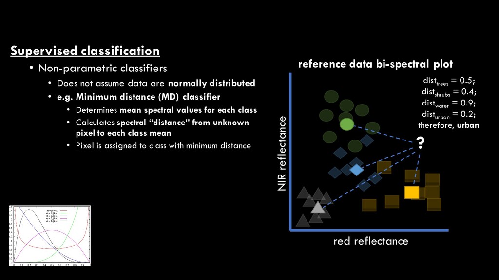
are normally distributed • e.g. Minimum distance (MD) classifier • Determines mean spectral values for each class • Calculates spectral “distance” from unknown pixel to each class mean • Pixel is assigned to class with minimum distance red reflectance NIR reflectance reference data bi-spectral plot ? disttrees = 0.5; distshrubs = 0.4; distwater = 0.9; disturban = 0.2; therefore, urban
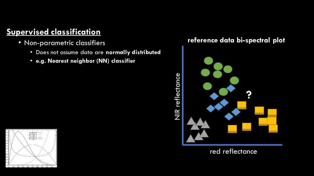
are normally distributed • e.g. Nearest neighbor (NN) classifier • Determines spectral “distance” from unknown pixel to every reference point red reflectance NIR reflectance reference data bi-spectral plot ?
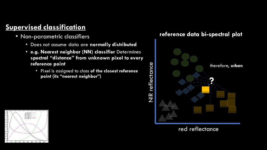
are normally distributed • e.g. Nearest neighbor (NN) classifier Determines spectral “distance” from unknown pixel to every reference point • Pixel is assigned to class of the closest reference point (its “nearest neighbor”) red reflectance NIR reflectance reference data bi-spectral plot ? therefore, urban
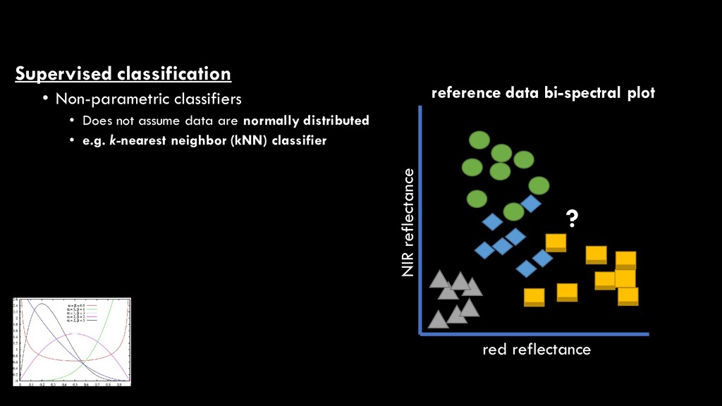
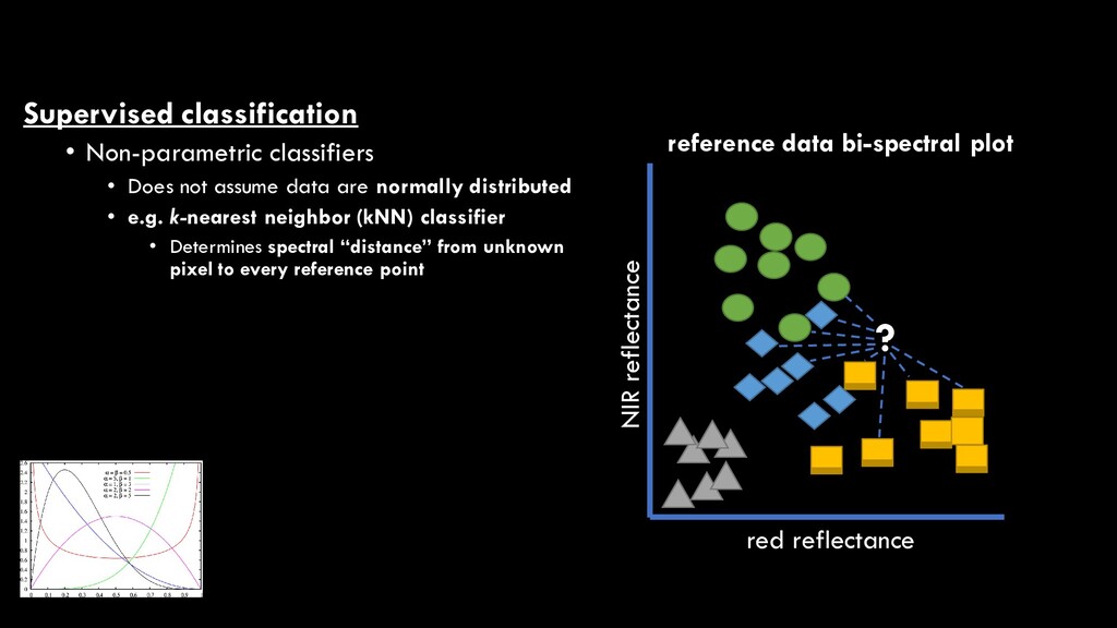
are normally distributed • e.g. k-nearest neighbor (kNN) classifier • Determines spectral “distance” from unknown pixel to every reference point red reflectance NIR reflectance reference data bi-spectral plot ?
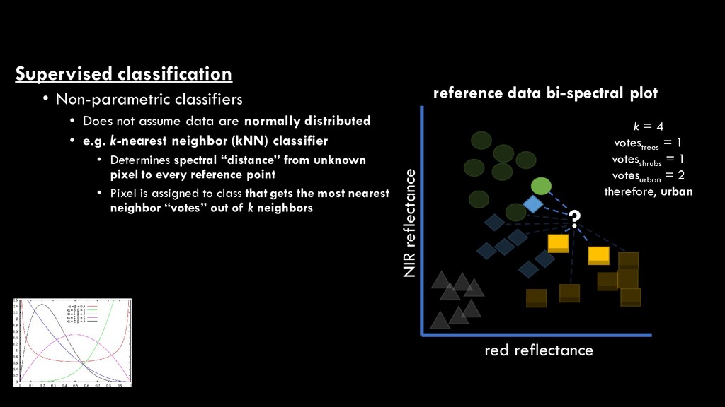
are normally distributed • e.g. k-nearest neighbor (kNN) classifier • Determines spectral “distance” from unknown pixel to every reference point • Pixel is assigned to class that gets the most nearest neighbor “votes” out of k neighbors red reflectance NIR reflectance reference data bi-spectral plot ? k = 4 votestrees = 1 votesshrubs = 1 votesurban = 2 therefore, urban
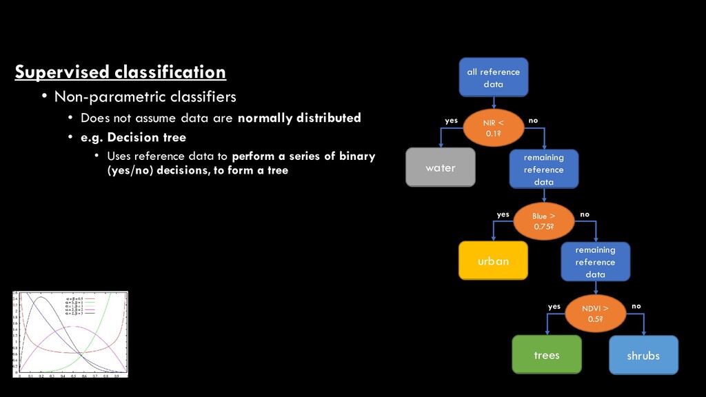
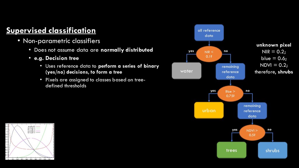
are normally distributed • e.g. Decision tree • Uses reference data to perform a series of binary (yes/no) decisions, to form a tree all reference data NIR < 0.1? water remaining reference data Blue > 0.75? urban remaining reference data NDVI > 0.5? trees shrubs yes no yes no yes no
are normally distributed • e.g. Decision tree • Uses reference data to perform a series of binary (yes/no) decisions, to form a tree • Pixels are assigned to classes based on tree- defined thresholds all reference data NIR < 0.1? water remaining reference data Blue > 0.75? urban remaining reference data NDVI > 0.5? trees shrubs yes no yes no yes no unknown pixel NIR = 0.2; blue = 0.6; NDVI = 0.2; therefore, shrubs
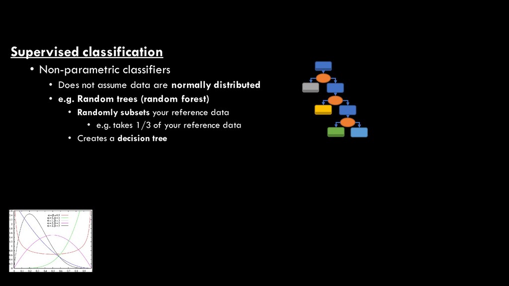
are normally distributed • e.g. Random trees (random forest) • Randomly subsets your reference data • e.g. takes 1/3 of your reference data • Creates a decision tree
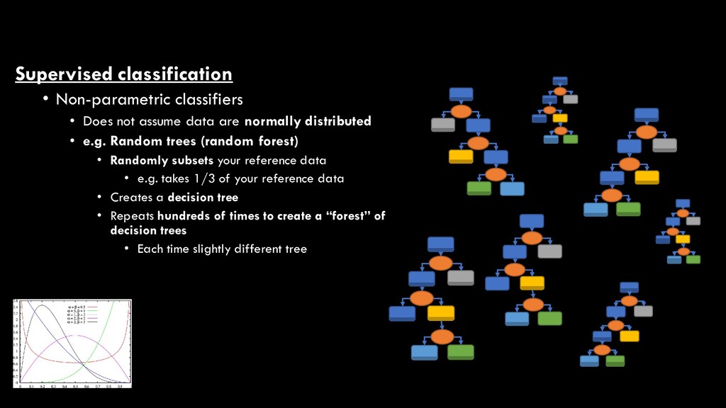
are normally distributed • e.g. Random trees (random forest) • Randomly subsets your reference data • e.g. takes 1/3 of your reference data • Creates a decision tree • Repeats hundreds of times to create a “forest” of decision trees • Each time slightly different tree
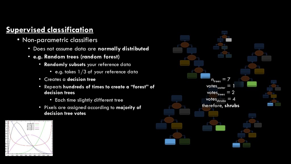
are normally distributed • e.g. Random trees (random forest) • Randomly subsets your reference data • e.g. takes 1/3 of your reference data • Creates a decision tree • Repeats hundreds of times to create a “forest” of decision trees • Each time slightly different tree • Pixels are assigned according to majority of decision tree votes ntrees = 7 voteswater = 1 votestrees = 2 votesshrubs = 4 therefore, shrubs
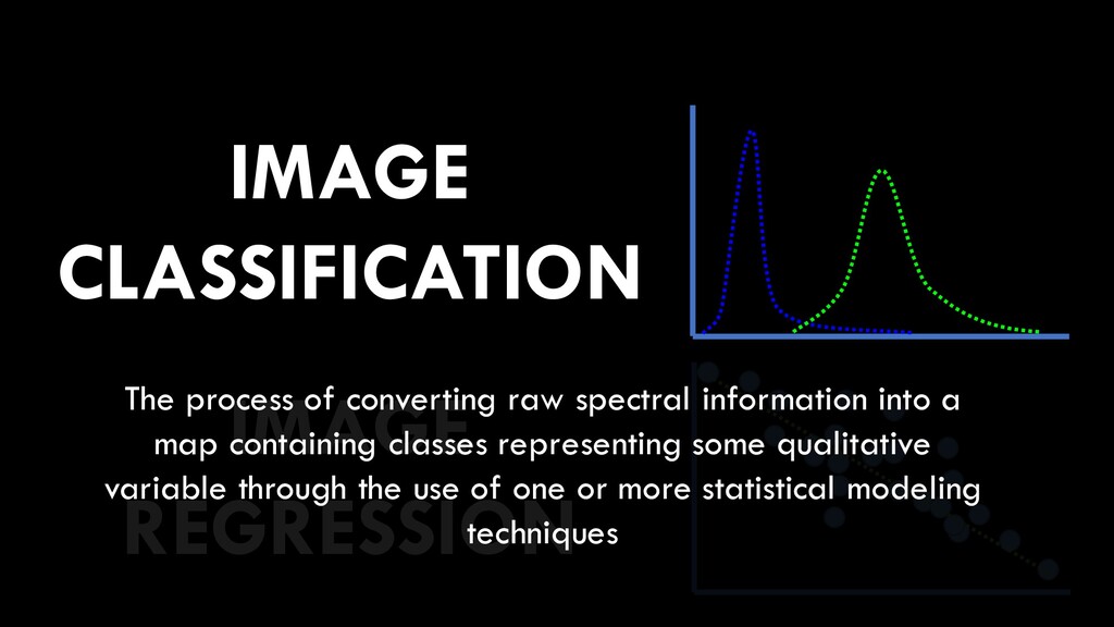
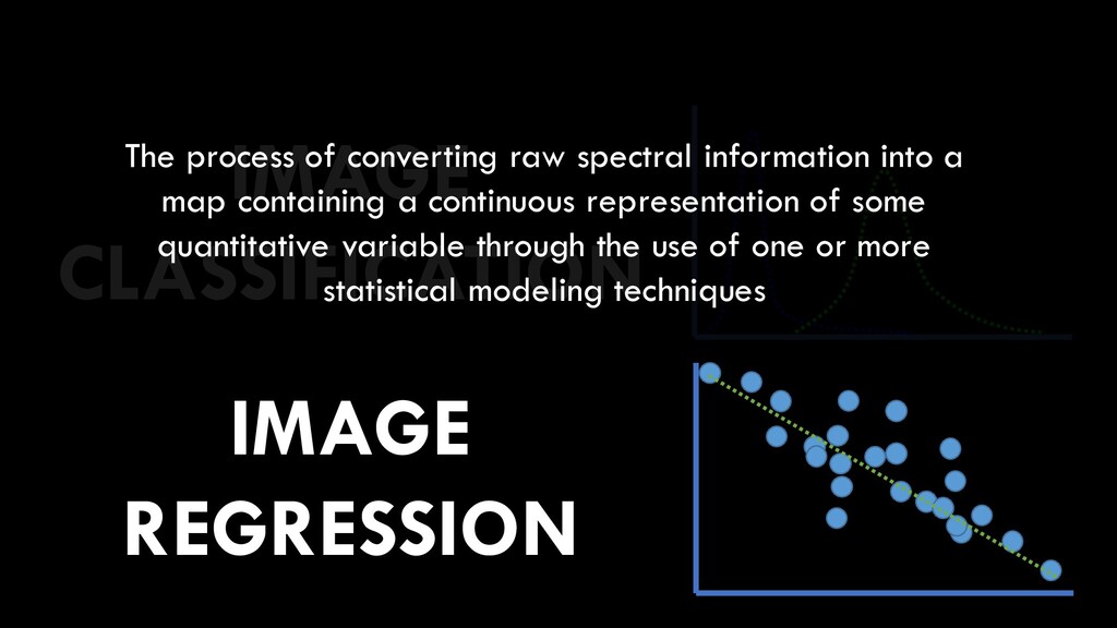
information into a map containing a continuous representation of some quantitative variable through the use of one or more statistical modeling techniques
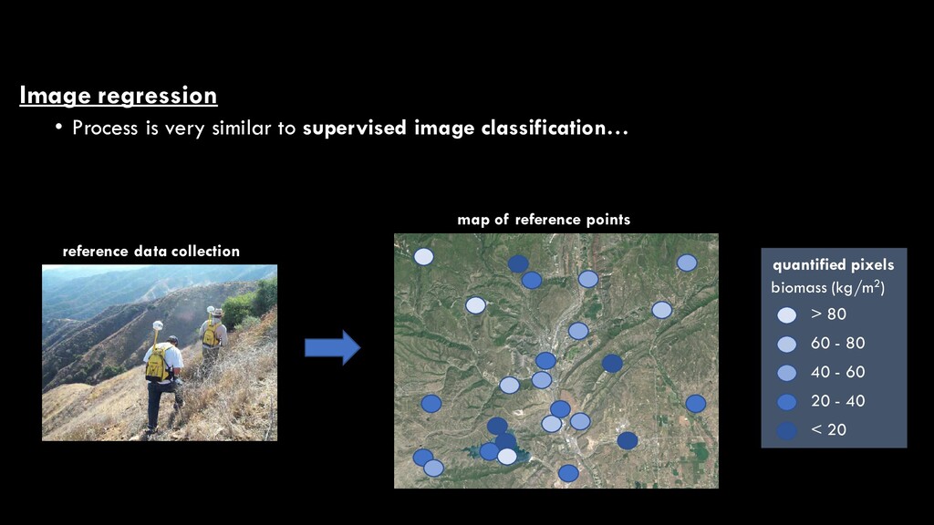
an image regression analysis is a map of some continuous variable • This is a supervised process • You need training data to derive the predictive regression model
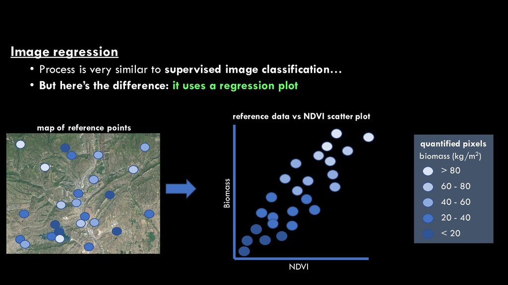
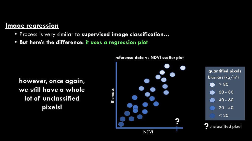
classification… • But here’s the difference: it uses a regression plot NDVI Biomass reference data vs NDVI scatter plot > 80 60 - 80 20 - 40 < 20 quantified pixels biomass (kg/m2) 40 - 60 however, once again, we still have a whole lot of unclassified pixels! ?unclassified pixel ?
classification… • But here’s the difference: it uses a regression plot NDVI Biomass reference data vs NDVI scatter plot > 80 60 - 80 20 - 40 < 20 quantified pixels biomass (kg/m2) 40 - 60 however, once again, we still have a whole lot of unclassified pixels! ?unclassified pixel ?
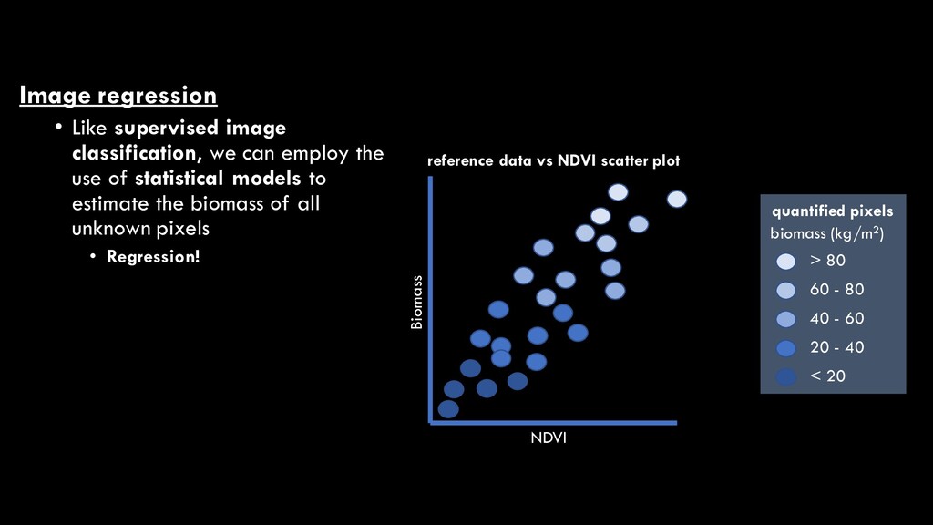
the use of statistical models to estimate the biomass of all unknown pixels • Regression! NDVI Biomass reference data vs NDVI scatter plot > 80 60 - 80 20 - 40 < 20 quantified pixels biomass (kg/m2) 40 - 60
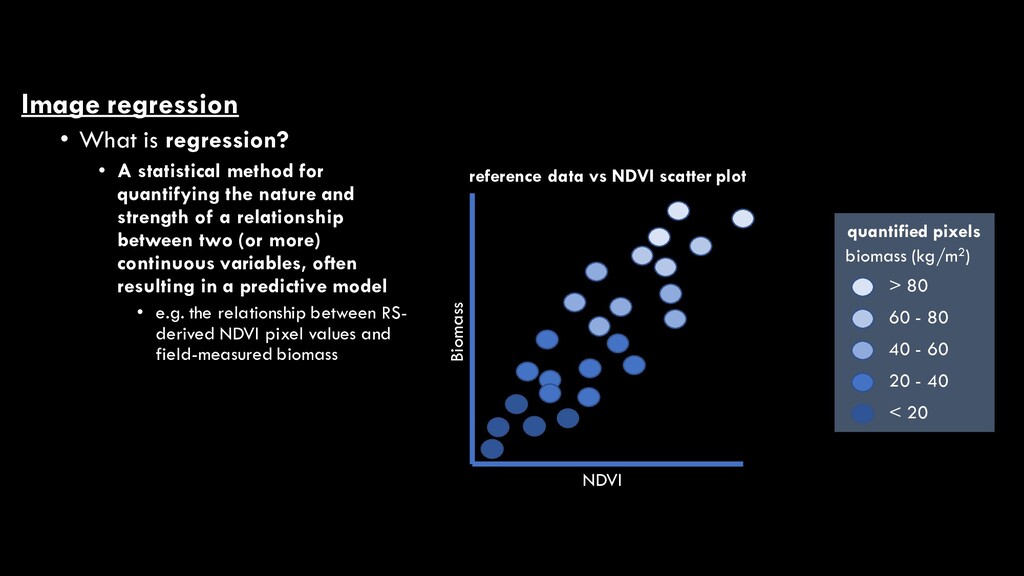
for quantifying the nature and strength of a relationship between two (or more) continuous variables, often resulting in a predictive model • e.g. the relationship between RS- derived NDVI pixel values and field-measured biomass NDVI Biomass reference data vs NDVI scatter plot > 80 60 - 80 20 - 40 < 20 quantified pixels biomass (kg/m2) 40 - 60
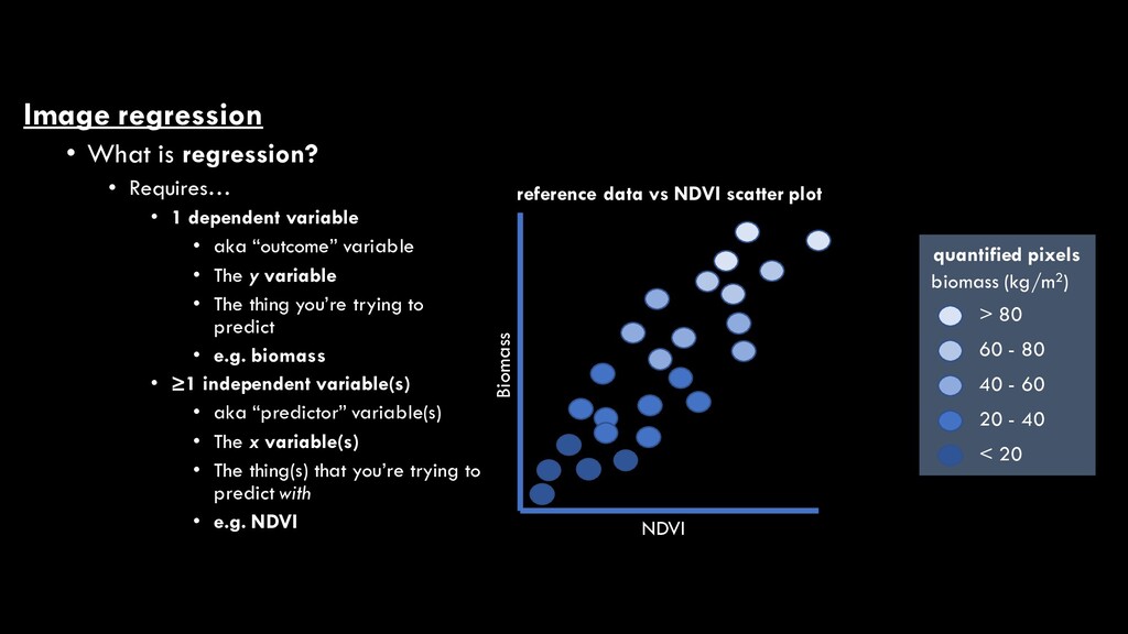
dependent variable • aka “outcome” variable • The y variable • The thing you’re trying to predict • e.g. biomass • ≥1 independent variable(s) • aka “predictor” variable(s) • The x variable(s) • The thing(s) that you’re trying to predict with • e.g. NDVI Biomass reference data vs NDVI scatter plot > 80 60 - 80 20 - 40 < 20 quantified pixels biomass (kg/m2) 40 - 60 NDVI
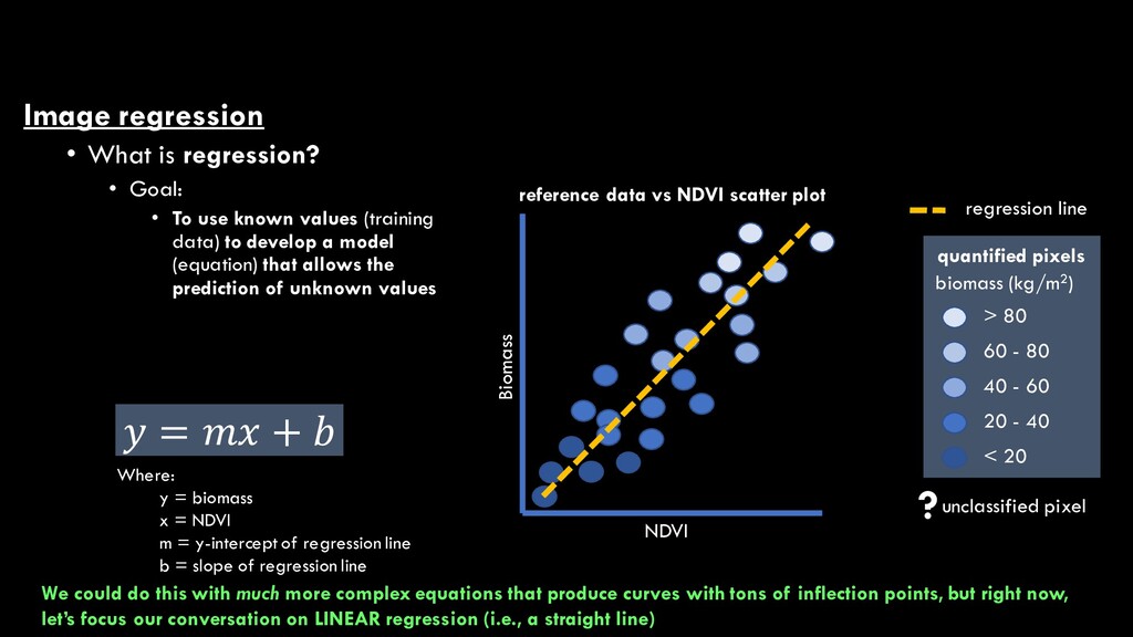
use known values (training data) to develop a model (equation) that allows the prediction of unknown values NDVI Biomass reference data vs NDVI scatter plot > 80 60 - 80 20 - 40 < 20 quantified pixels biomass (kg/m2) 40 - 60 ?unclassified pixel regression line 𝑦𝑦 = 𝑚𝑚𝑚𝑚 + 𝑏𝑏 Where: y = biomass x = NDVI m = y-intercept of regression line b = slope of regression line
use known values (training data) to develop a model (equation) that allows the prediction of unknown values NDVI Biomass reference data vs NDVI scatter plot > 80 60 - 80 20 - 40 < 20 quantified pixels biomass (kg/m2) 40 - 60 ?unclassified pixel regression line 𝑦𝑦 = 𝑚𝑚𝑚𝑚 + 𝑏𝑏 Where: y = biomass x = NDVI m = y-intercept of regression line b = slope of regression line We could do this with much more complex equations that produce curves with tons of inflection points, but right now, let’s focus our conversation on LINEAR regression (i.e., a straight line)
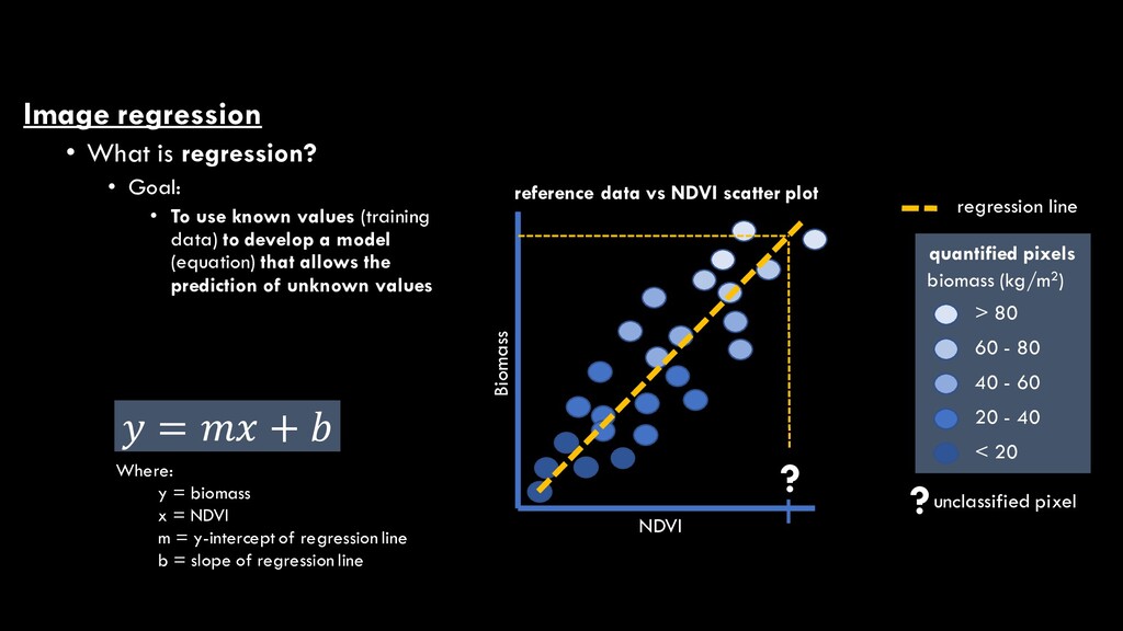
use known values (training data) to develop a model (equation) that allows the prediction of unknown values NDVI Biomass reference data vs NDVI scatter plot > 80 60 - 80 20 - 40 < 20 quantified pixels biomass (kg/m2) 40 - 60 ?unclassified pixel regression line 𝑦𝑦 = 𝑚𝑚𝑚𝑚 + 𝑏𝑏 Where: y = biomass x = NDVI m = y-intercept of regression line b = slope of regression line ?
use known values (training data) to develop a model (equation) that allows the prediction of unknown values NDVI Biomass reference data vs NDVI scatter plot > 80 60 - 80 20 - 40 < 20 quantified pixels biomass (kg/m2) 40 - 60 ?unclassified pixel regression line ? 𝑦𝑦 = 𝑚𝑚𝑚𝑚 + 𝑏𝑏 Where: y = biomass x = NDVI m = y-intercept of regression line b = slope of regression line
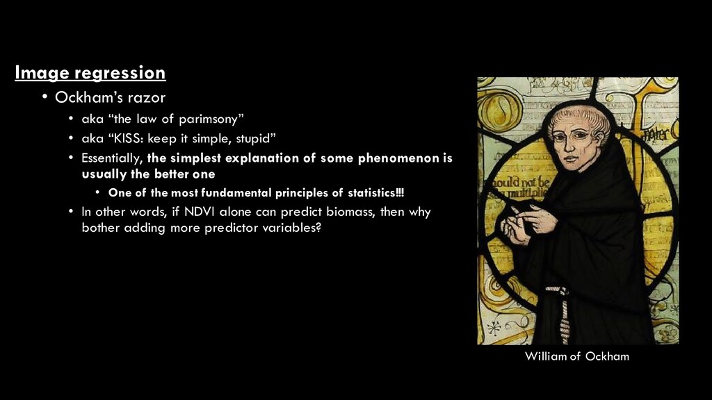
parimsony” • aka “KISS: keep it simple, stupid” • Essentially, the simplest explanation of some phenomenon is usually the better one • One of the most fundamental principles of statistics!!! • In other words, if NDVI alone can predict biomass, then why bother adding more predictor variables? William of Ockham
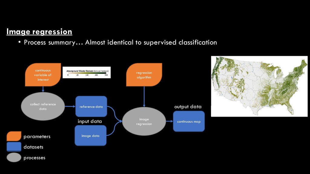
image data image regression continuous map regression algorithm input data output data parameters datasets processes reference data continuous variable of interest collect reference data