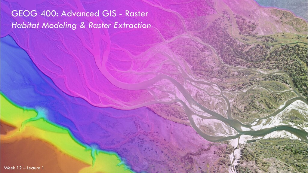
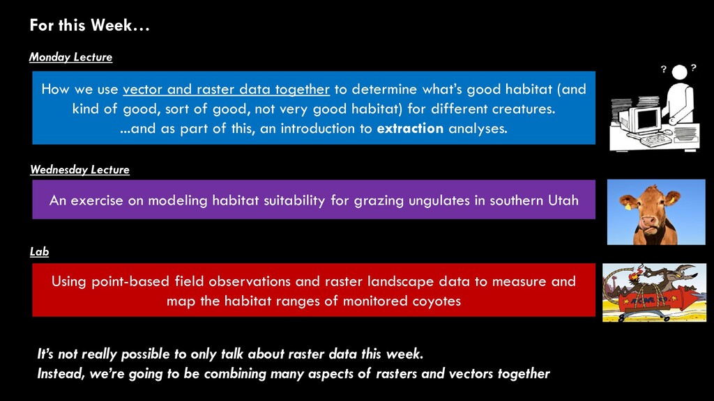
what’s good habitat (and kind of good, sort of good, not very good habitat) for different creatures. ...and as part of this, an introduction to extraction analyses. An exercise on modeling habitat suitability for grazing ungulates in southern Utah For this Week… Monday Lecture Wednesday Lecture Lab Using point-based field observations and raster landscape data to measure and map the habitat ranges of monitored coyotes It’s not really possible to only talk about raster data this week. Instead, we’re going to be combining many aspects of rasters and vectors together
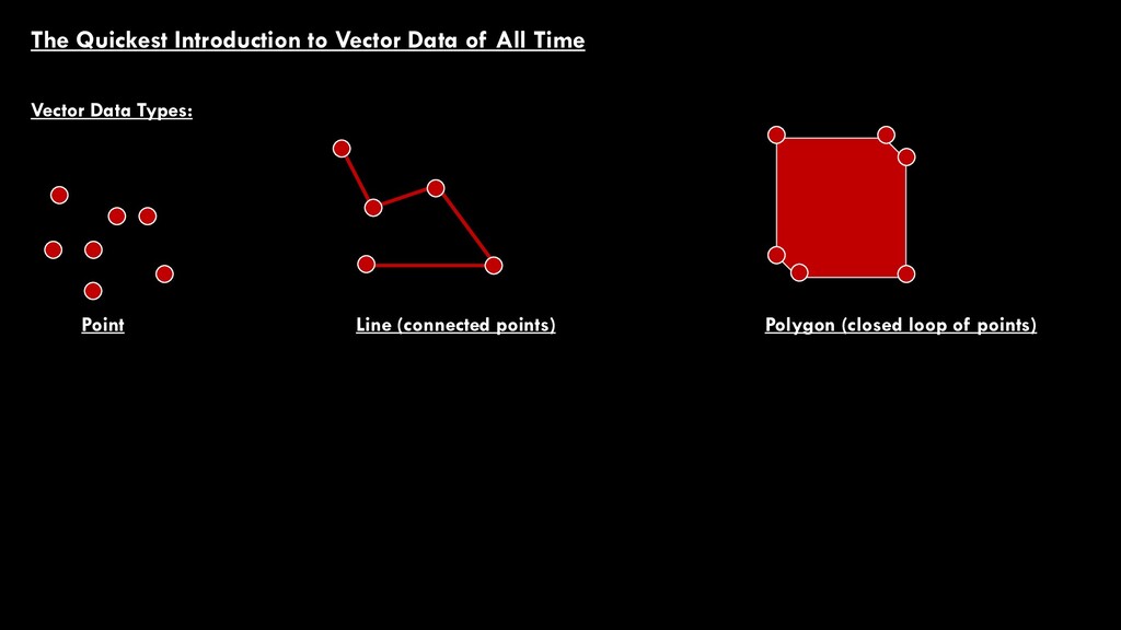
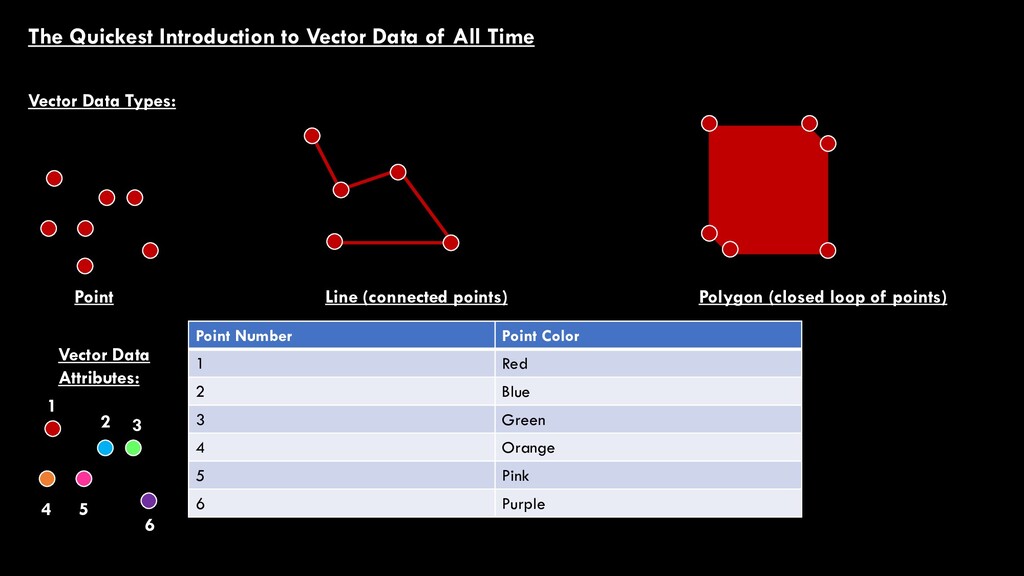
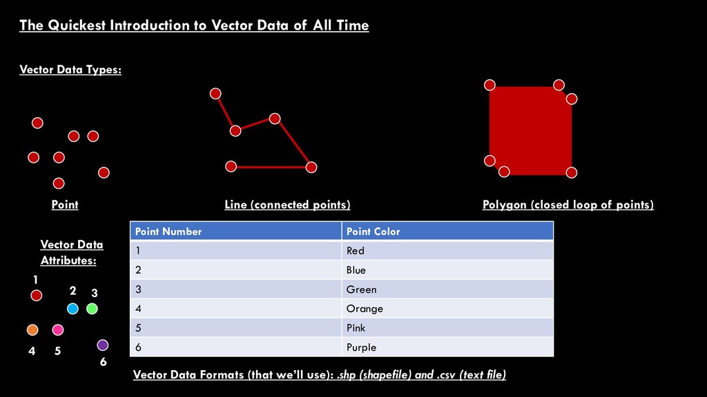
Data Types: Point Line (connected points) Polygon (closed loop of points) 1 2 3 4 5 6 Point Number Point Color 1 Red 2 Blue 3 Green 4 Orange 5 Pink 6 Purple Vector Data Attributes:
Data Types: Point Line (connected points) Polygon (closed loop of points) 1 2 3 4 5 6 Point Number Point Color 1 Red 2 Blue 3 Green 4 Orange 5 Pink 6 Purple Vector Data Attributes: Vector Data Formats (that we’ll use): .shp (shapefile) and .csv (text file)
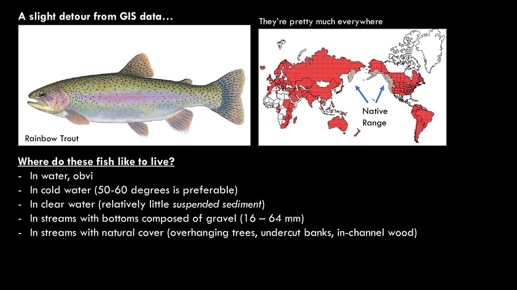
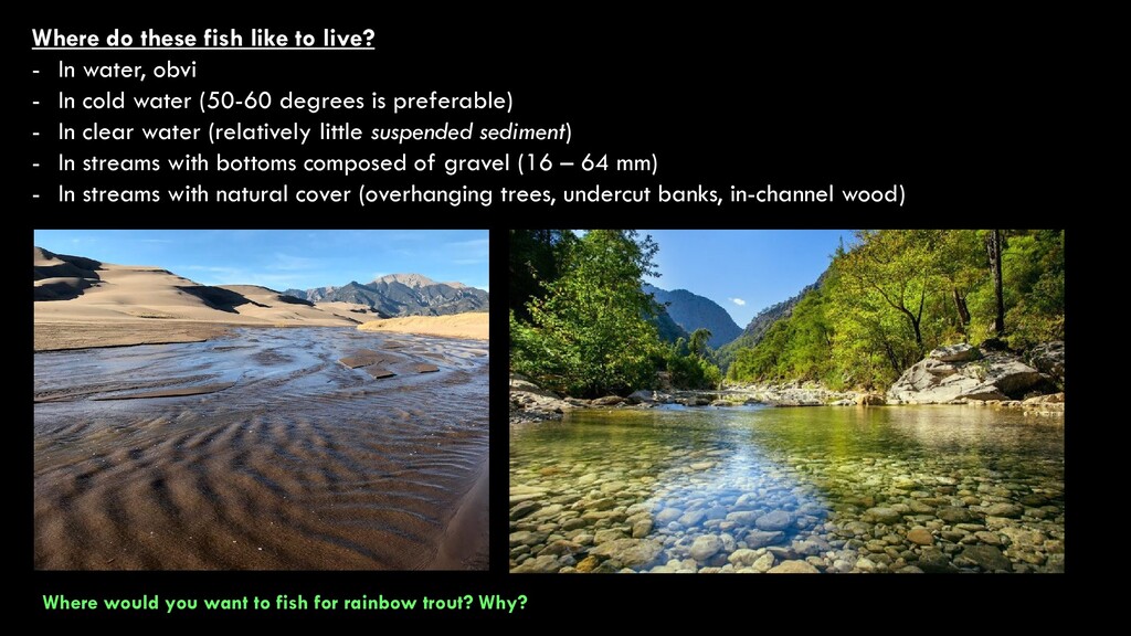
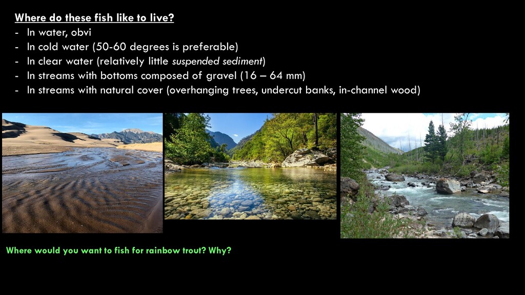
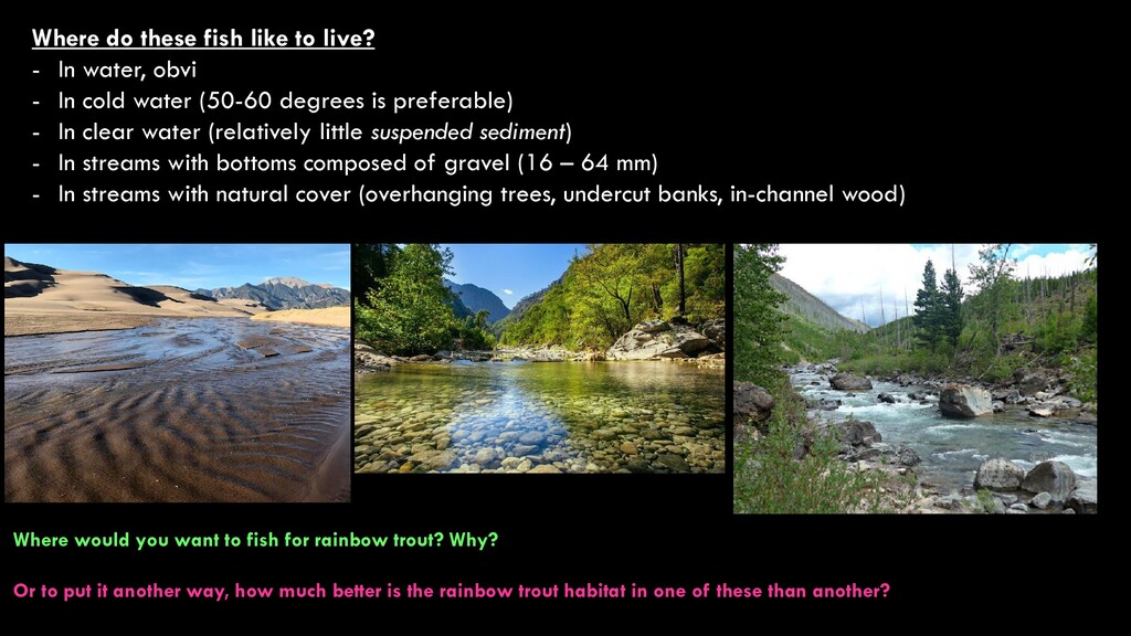
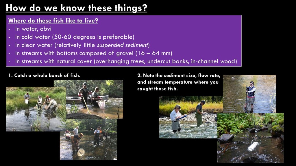
They’re pretty much everywhere Where do these fish like to live? - In water, obvi - In cold water (50-60 degrees is preferable) - In clear water (relatively little suspended sediment) - In streams with bottoms composed of gravel (16 – 64 mm) - In streams with natural cover (overhanging trees, undercut banks, in-channel wood)
obvi - In cold water (50-60 degrees is preferable) - In clear water (relatively little suspended sediment) - In streams with bottoms composed of gravel (16 – 64 mm) - In streams with natural cover (overhanging trees, undercut banks, in-channel wood) Where would you want to fish for rainbow trout? Why?
obvi - In cold water (50-60 degrees is preferable) - In clear water (relatively little suspended sediment) - In streams with bottoms composed of gravel (16 – 64 mm) - In streams with natural cover (overhanging trees, undercut banks, in-channel wood) Where would you want to fish for rainbow trout? Why?
obvi - In cold water (50-60 degrees is preferable) - In clear water (relatively little suspended sediment) - In streams with bottoms composed of gravel (16 – 64 mm) - In streams with natural cover (overhanging trees, undercut banks, in-channel wood) Where would you want to fish for rainbow trout? Why? Or to put it another way, how much better is the rainbow trout habitat in one of these than another?
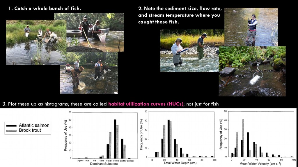
obvi - In cold water (50-60 degrees is preferable) - In clear water (relatively little suspended sediment) - In streams with bottoms composed of gravel (16 – 64 mm) - In streams with natural cover (overhanging trees, undercut banks, in-channel wood) How do we know these things? 1. Catch a whole bunch of fish. 2. Note the sediment size, flow rate, and stream temperature where you caught those fish.
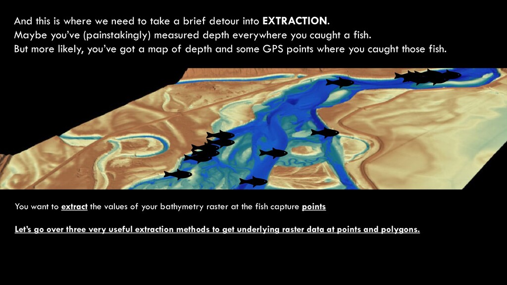
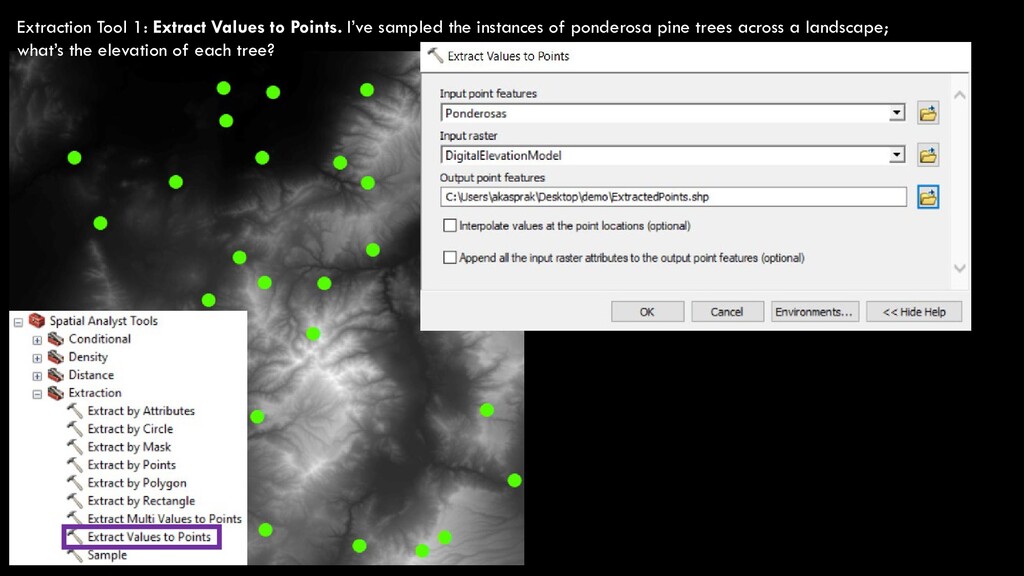
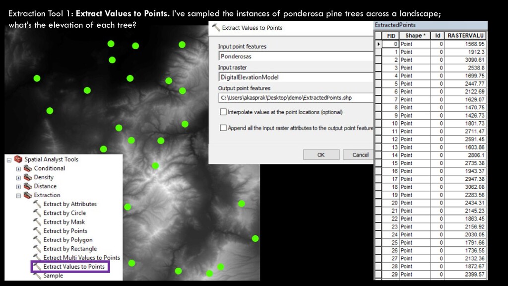
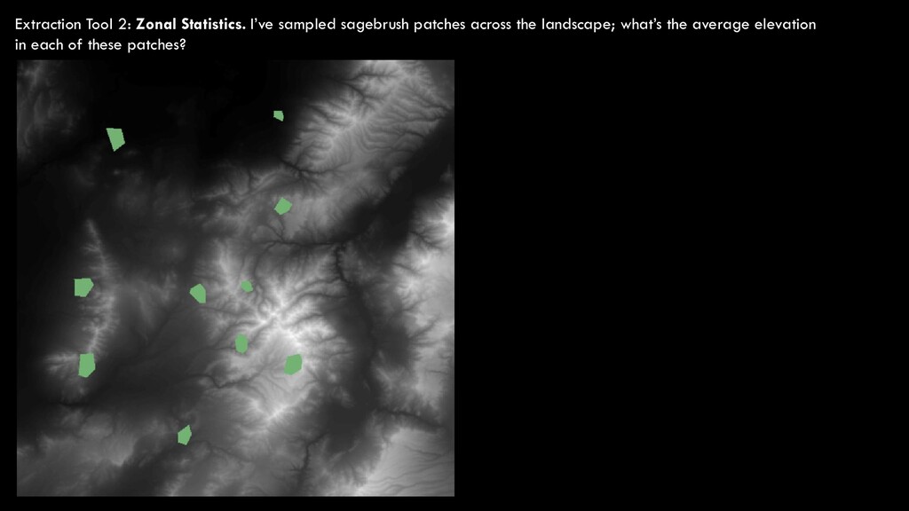
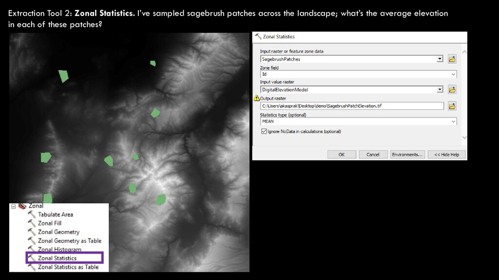
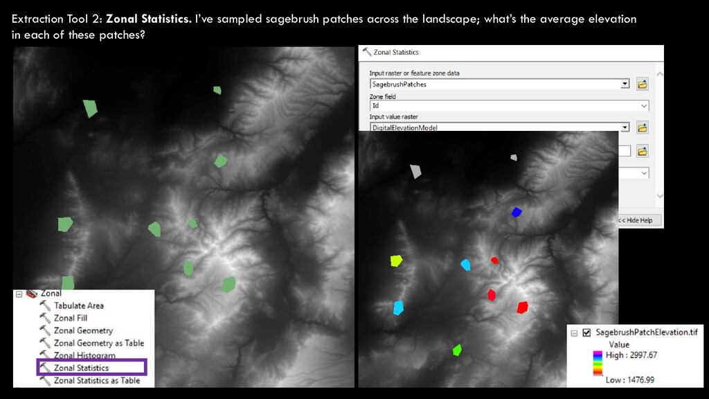
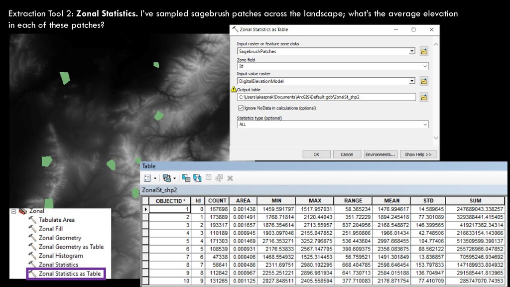
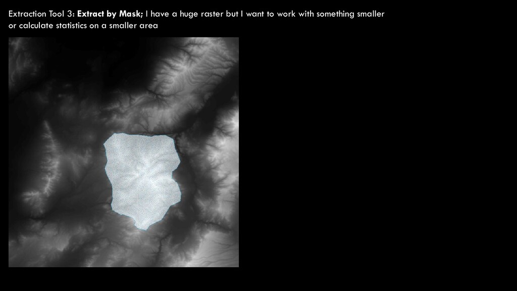
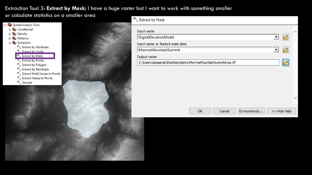
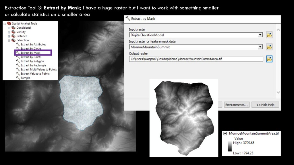
detour into EXTRACTION. Maybe you’ve (painstakingly) measured depth everywhere you caught a fish. But more likely, you’ve got a map of depth and some GPS points where you caught those fish. You want to extract the values of your bathymetry raster at the fish capture points Let’s go over three very useful extraction methods to get underlying raster data at points and polygons.
obvi - In cold water (50-60 degrees is preferable) - In clear water (relatively little suspended sediment) - In streams with bottoms composed of gravel (16 – 64 mm) - In streams with natural cover (overhanging trees, undercut banks, in-channel wood) How do we know these things? 1. Catch a whole bunch of fish. 2. Note the sediment size, flow rate, and stream temperature where you caught those fish.
sediment size, flow rate, and stream temperature where you caught those fish. 3. Plot these up as histograms; these are called habitat utilization curves (HUCs); not just for fish
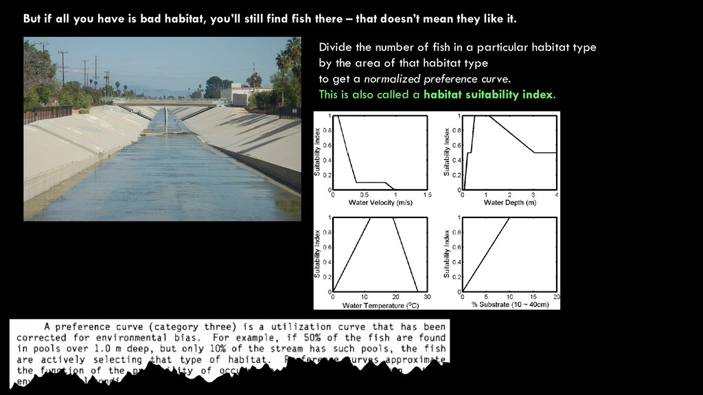
find fish there – that doesn’t mean they like it. Divide the number of fish in a particular habitat type by the area of that habitat type to get a normalized preference curve. This is also called a habitat suitability index.
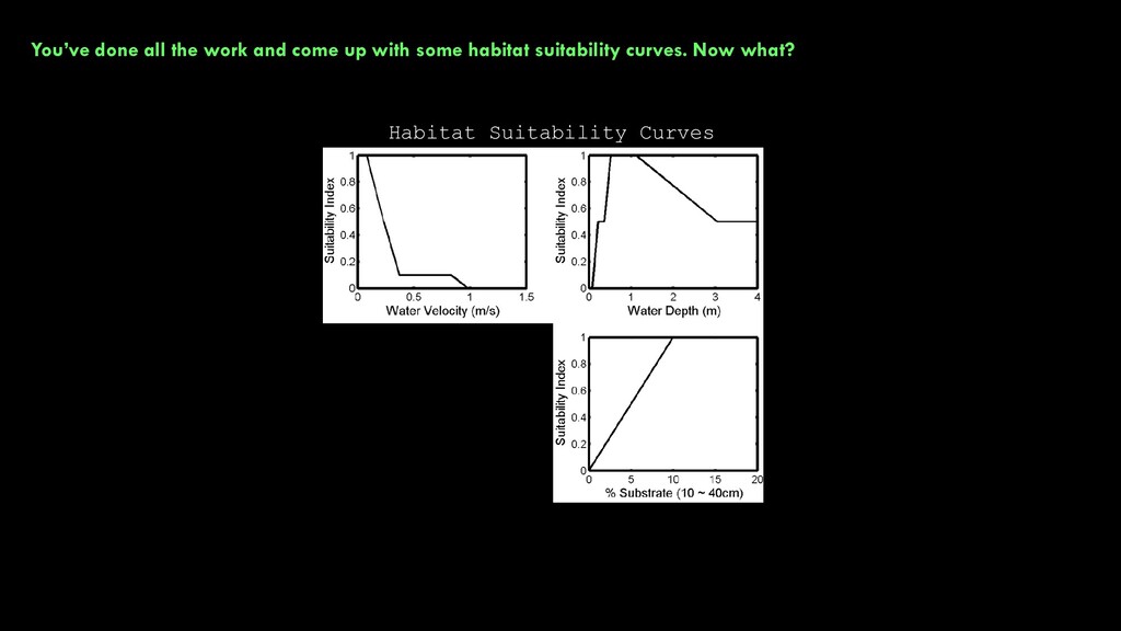
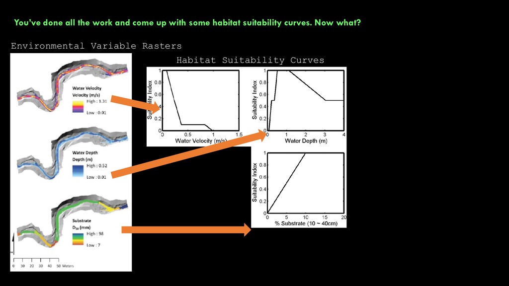
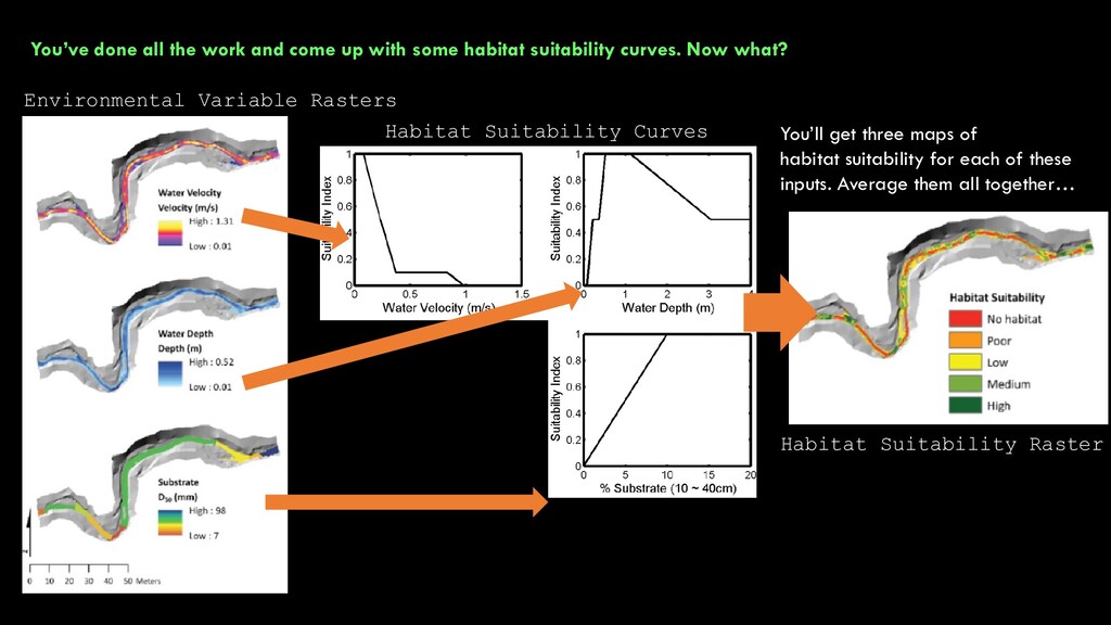
habitat suitability curves. Now what? You’ll get three maps of habitat suitability for each of these inputs. Average them all together… Habitat Suitability Curves Environmental Variable Rasters Habitat Suitability Raster
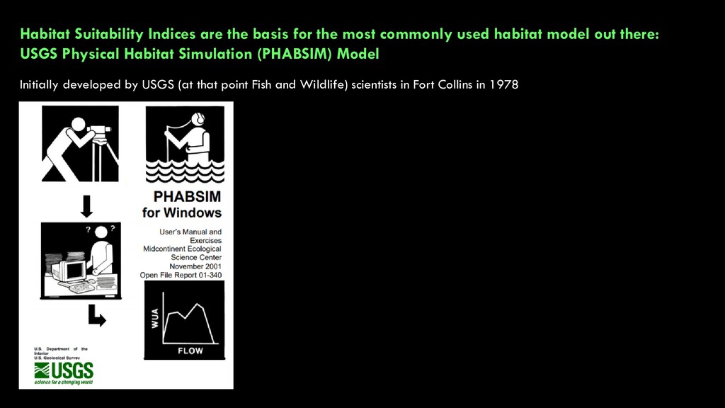
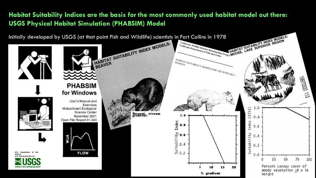
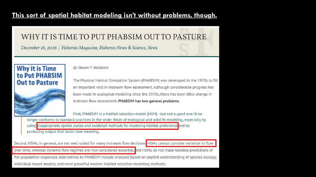
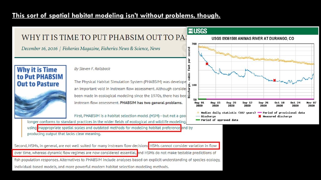
used habitat model out there: USGS Physical Habitat Simulation (PHABSIM) Model Initially developed by USGS (at that point Fish and Wildlife) scientists in Fort Collins in 1978
used habitat model out there: USGS Physical Habitat Simulation (PHABSIM) Model Initially developed by USGS (at that point Fish and Wildlife) scientists in Fort Collins in 1978
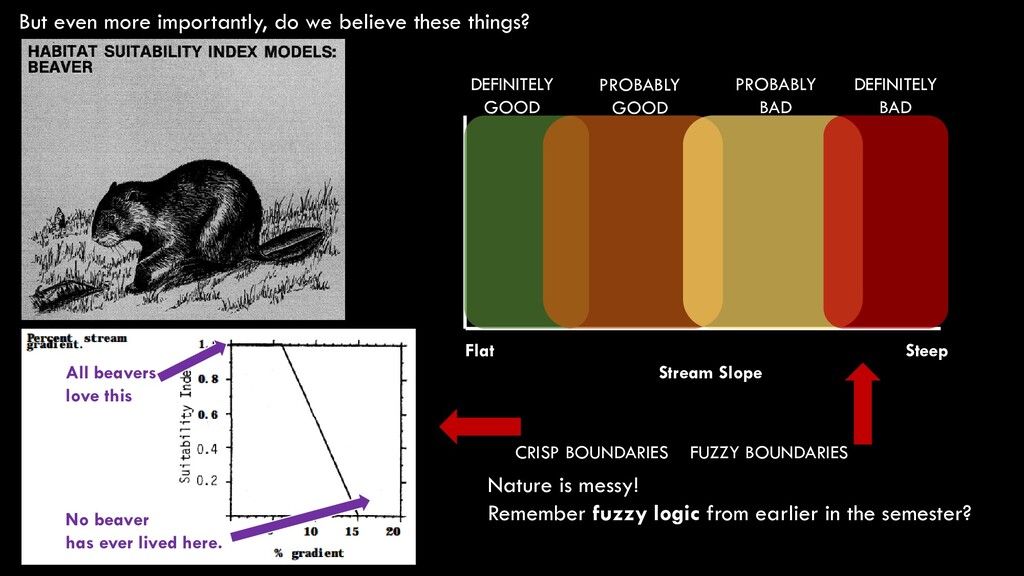
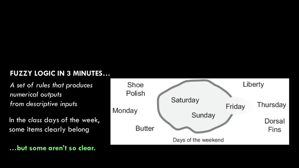
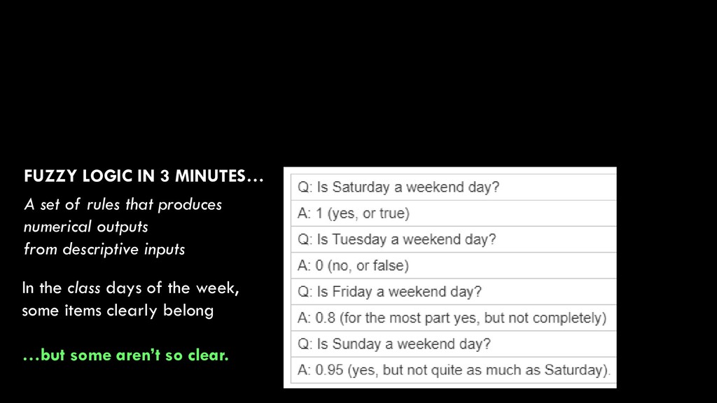
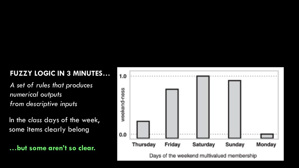
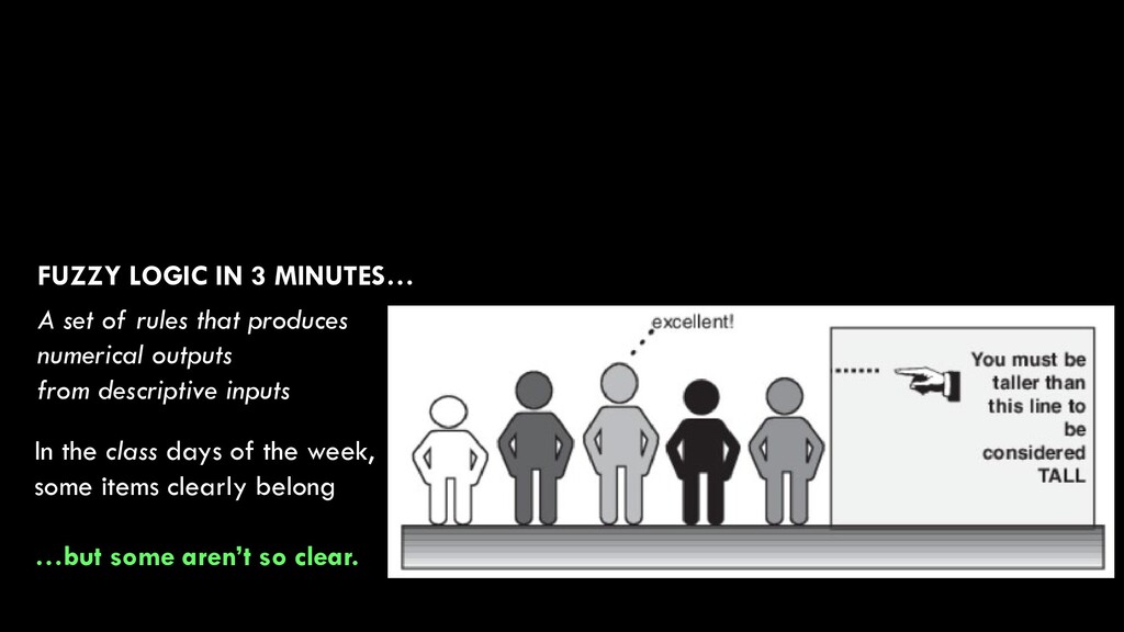
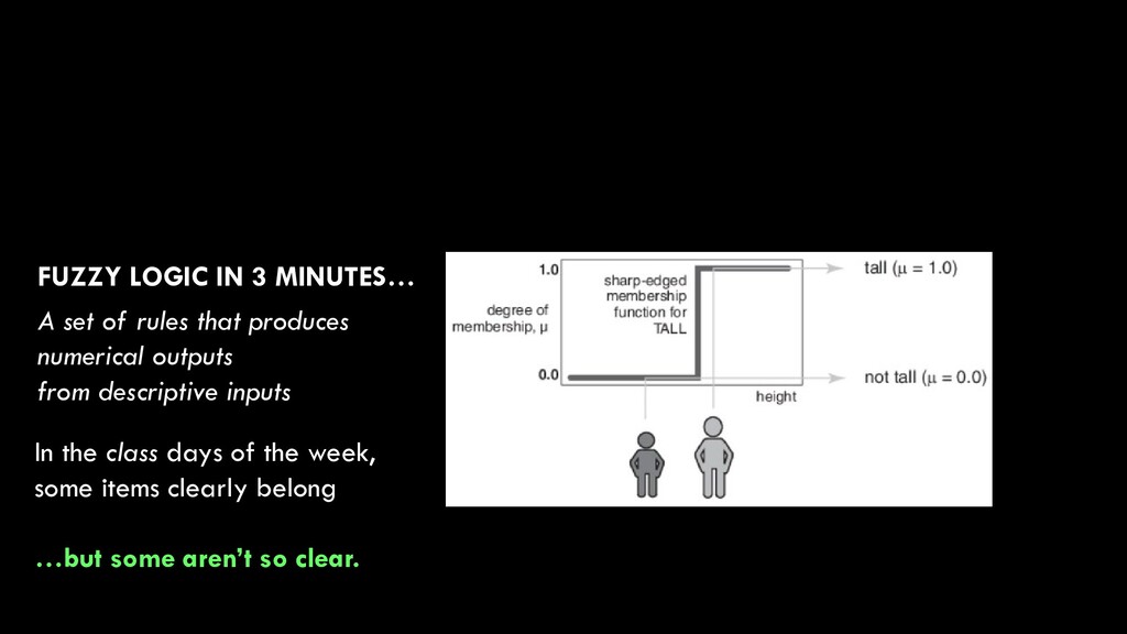
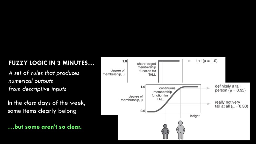
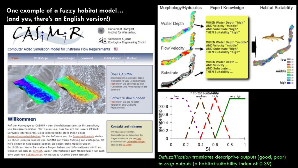
beavers love this No beaver has ever lived here. Stream Slope Flat Steep DEFINITELY GOOD PROBABLY GOOD PROBABLY BAD DEFINITELY BAD Nature is messy! Remember fuzzy logic from earlier in the semester? CRISP BOUNDARIES FUZZY BOUNDARIES
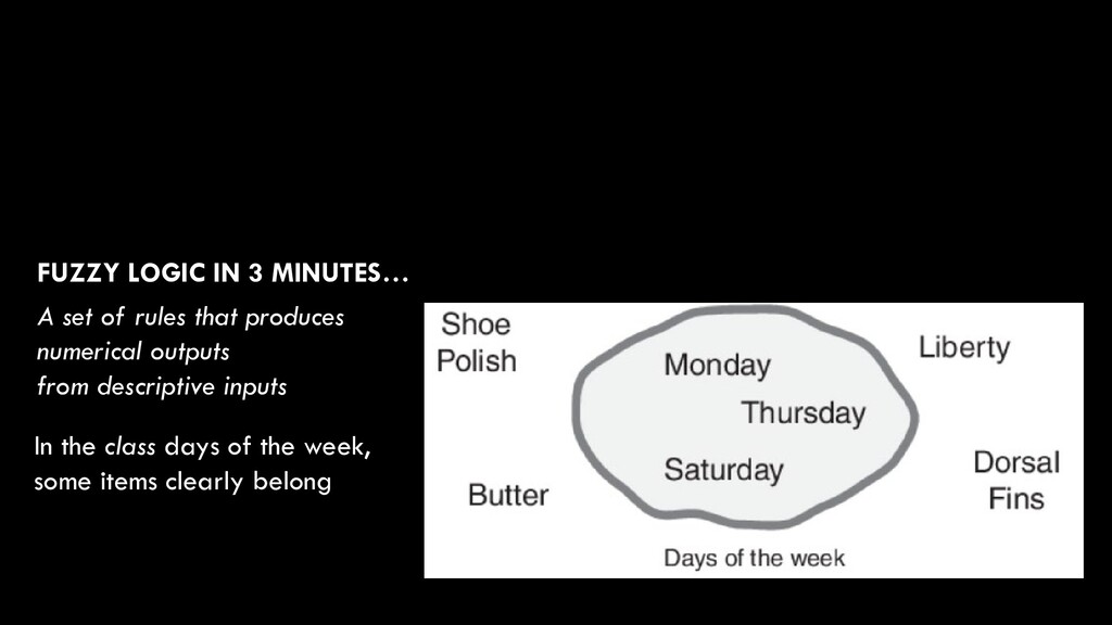
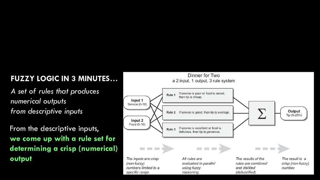
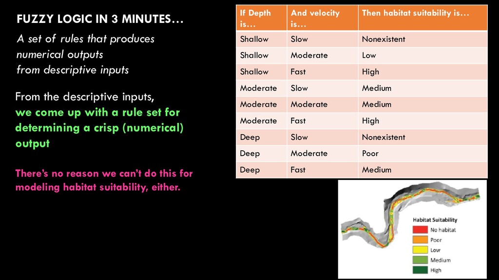
produces numerical outputs from descriptive inputs From the descriptive inputs, we come up with a rule set for determining a crisp (numerical) output There’s no reason we can’t do this for modeling habitat suitability, either. If Depth is… And velocity is… Then habitat suitability is… Shallow Slow Nonexistent Shallow Moderate Low Shallow Fast High Moderate Slow Medium Moderate Moderate Medium Moderate Fast High Deep Slow Nonexistent Deep Moderate Poor Deep Fast Medium
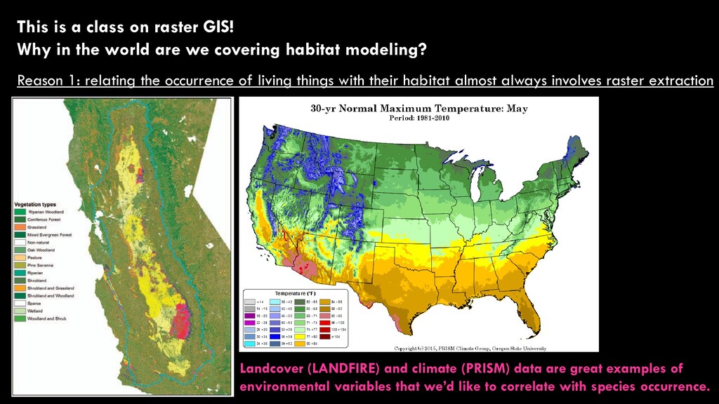
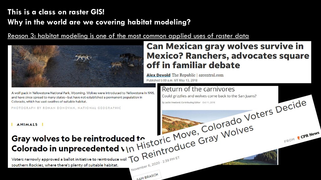
world are we covering habitat modeling? Reason 1: relating the occurrence of living things with their habitat almost always involves raster extraction Landcover (LANDFIRE) and climate (PRISM) data are great examples of environmental variables that we’d like to correlate with species occurrence.
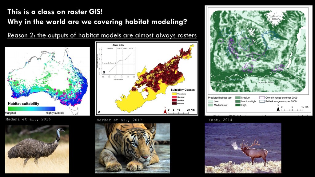
world are we covering habitat modeling? Reason 2: the outputs of habitat models are almost always rasters Madani et al., 2016 Sarkar et al., 2017 Yost, 2014