Phylogenetic diversity indices (not only) in metagenomics

Research Group on Natural Computing Seminar, University of Seville, 16-06-2014

Transcript

1. Phylogenetic diversity indices (not only) in metagenomics Francesc Rosselló Computational Biology and Bioinformatics Research Group, UIB Sevilla, June 16, 2014
2. Biodiversity • Biodiversity is the biology of numbers and difference (K. J. Gaston, 1996) • Biodiversity is what biodiversity indices measure 2 / 40
3. Biodiversity and conservation Understanding evolution http://evolution.berkeley.edu 3 / 40
4. Comparative metagenomics Comparative metagenomics studies compositional patterns within microbial communities and compares patterns between communities 10% of cells in a person are human E. Grice, Science 324 (2009), 1190–1192 4 / 40
5. Comparative metagenomics Comparative metagenomics studies compositional patterns within microbial communities and compares patterns between communities H. Jakobsson, PLoS ONE 5 (2010): e9836 5 / 40
6. Comparative metagenomics Comparative metagenomics studies compositional patterns within microbial communities and compares patterns between communities O. Koren, PLoS Comput Biol 9 (2013): e1002863 6 / 40
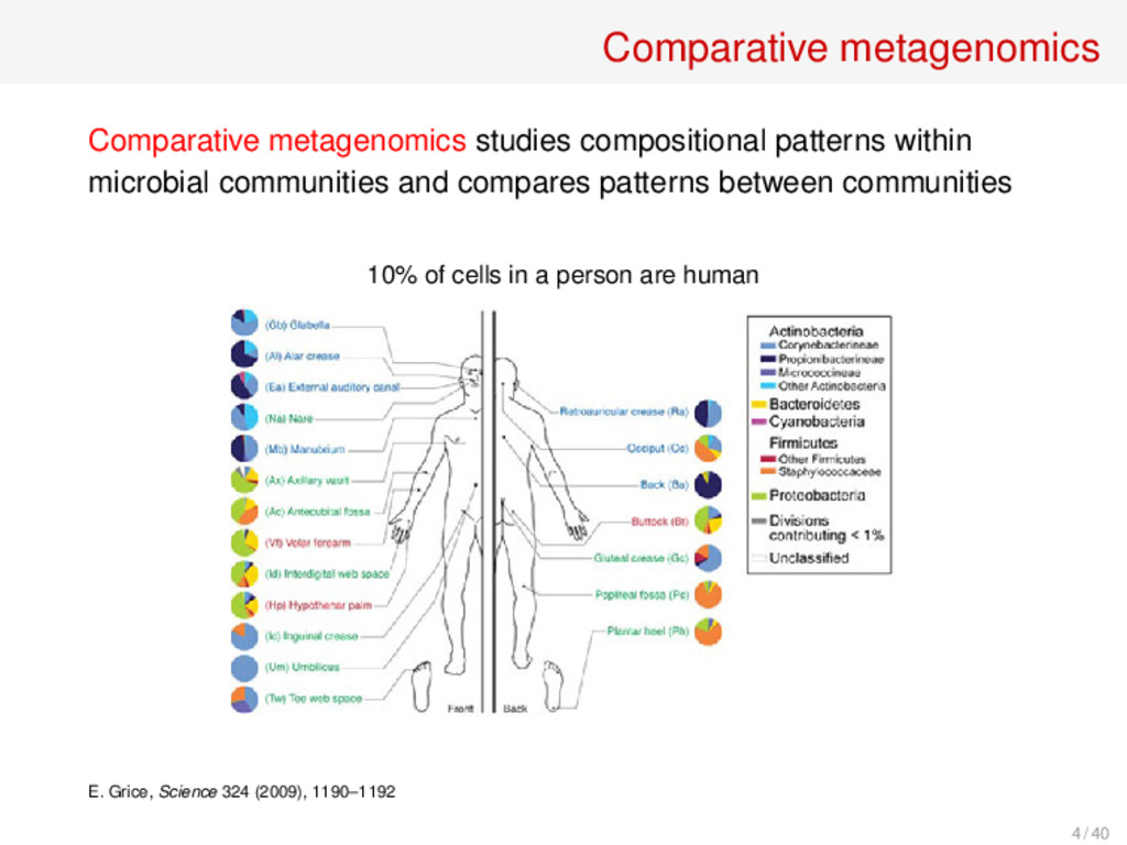
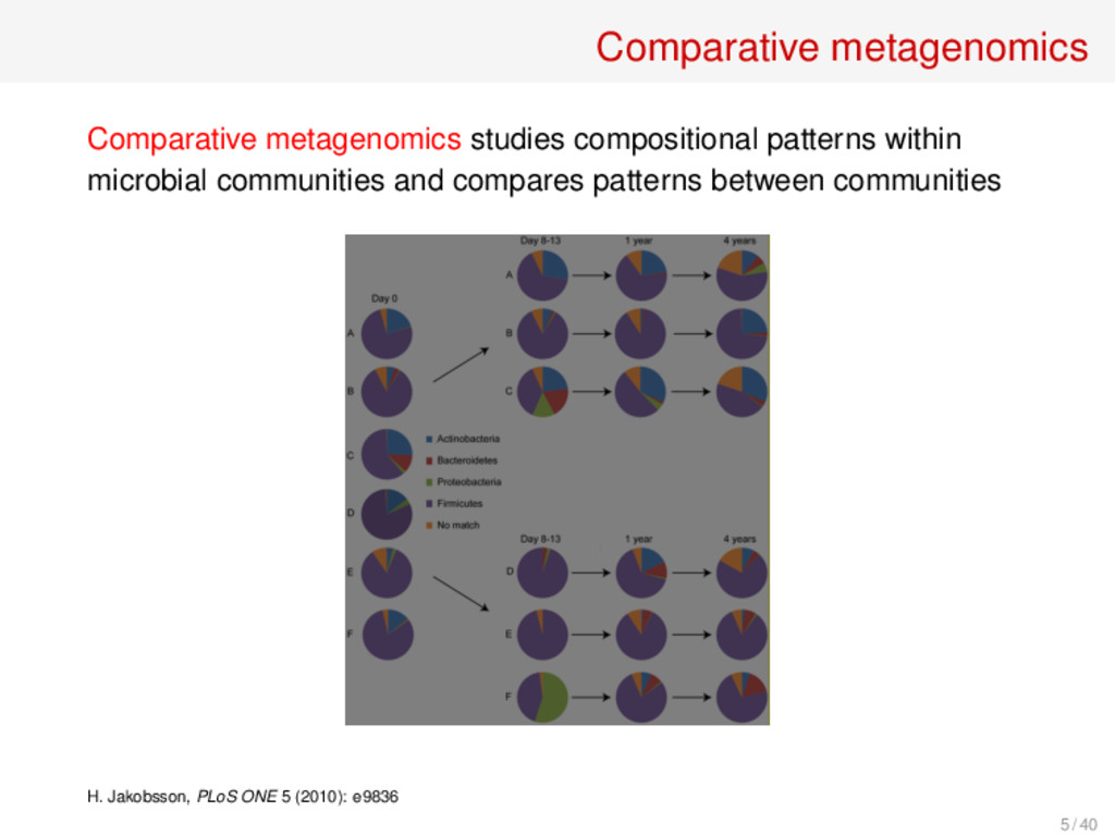
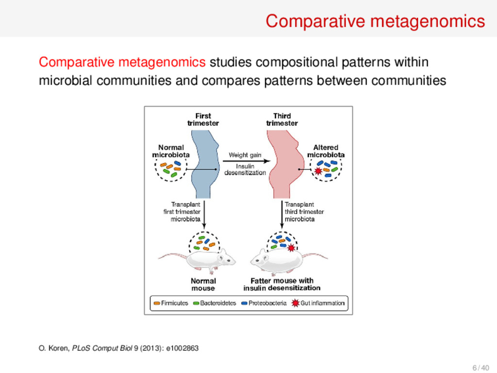
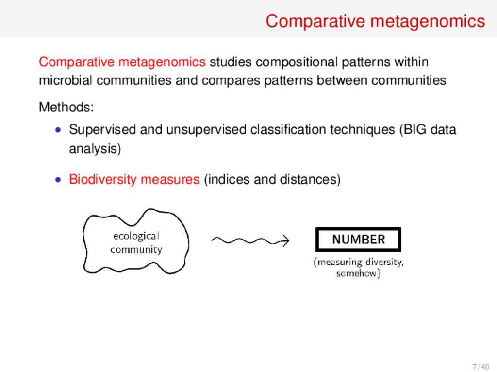
7. Comparative metagenomics Comparative metagenomics studies compositional patterns within microbial communities and compares patterns between communities Methods: • Supervised and unsupervised classification techniques (BIG data analysis) • Biodiversity measures (indices and distances) 7 / 40
8. Outline Biodiversity indices ⇓ Phylogenetic biodiversity indices ⇓ Community phylogenetic comparison 8 / 40
9. Secondary goal 9 / 40
10. Biodiversity indices Biodiversity indices try to measure: Richness: Number of species in a community Homogeneity: Evenness of species in a community Which one is more diverse? 10 / 40
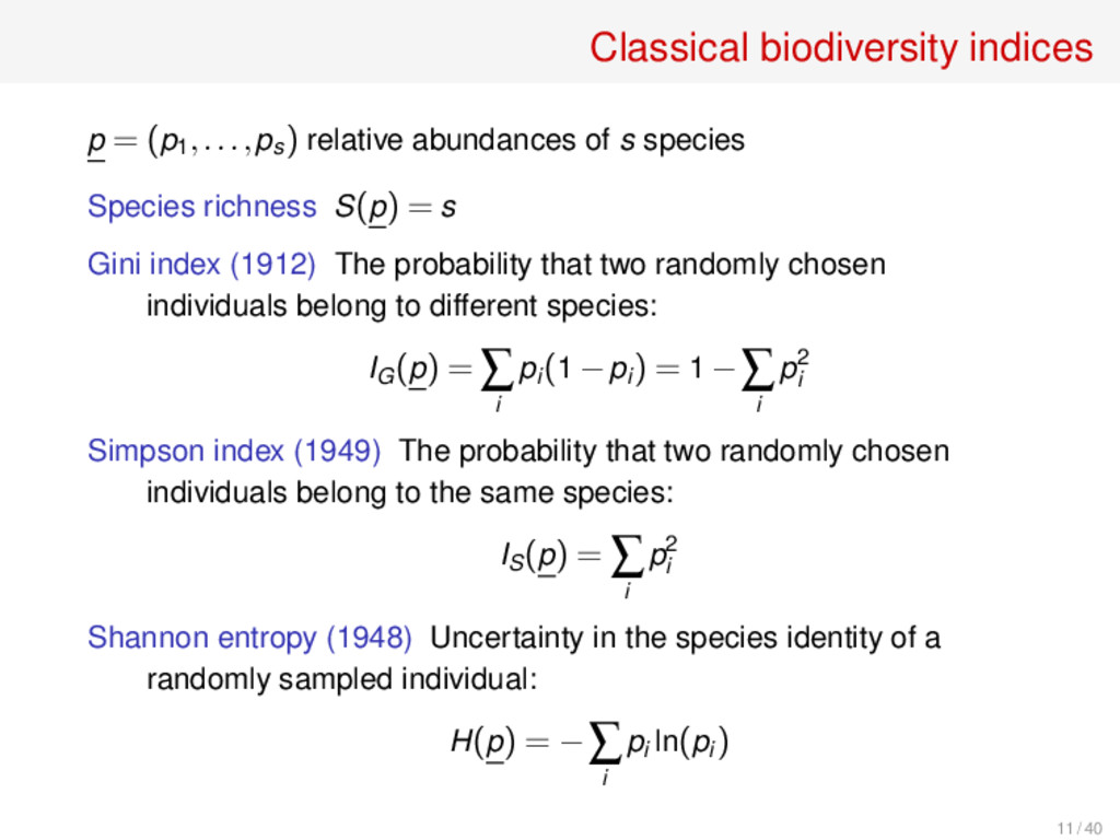
11. Classical biodiversity indices p = (p1 ,...,ps ) relative abundances of s species Species richness S(p) = s Gini index (1912) The probability that two randomly chosen individuals belong to different species: IG (p) = ∑ i pi (1 −pi ) = 1 −∑ i p2 i Simpson index (1949) The probability that two randomly chosen individuals belong to the same species: IS (p) = ∑ i p2 i Shannon entropy (1948) Uncertainty in the species identity of a randomly sampled individual: H(p) = −∑ i pi ln(pi ) 11 / 40
12. Classical biodiversity indices Which one is more diverse? S = 4 S = 3 IG = 0.531 IG = 0.667 H = 1.003 H = 1.099 12 / 40
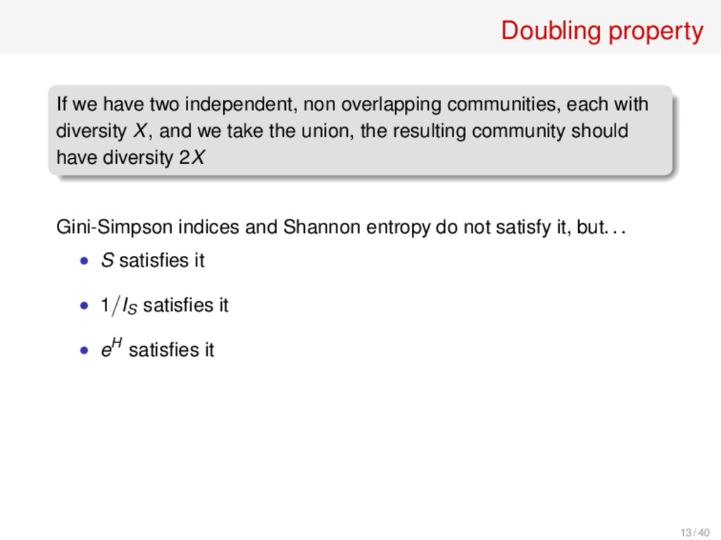
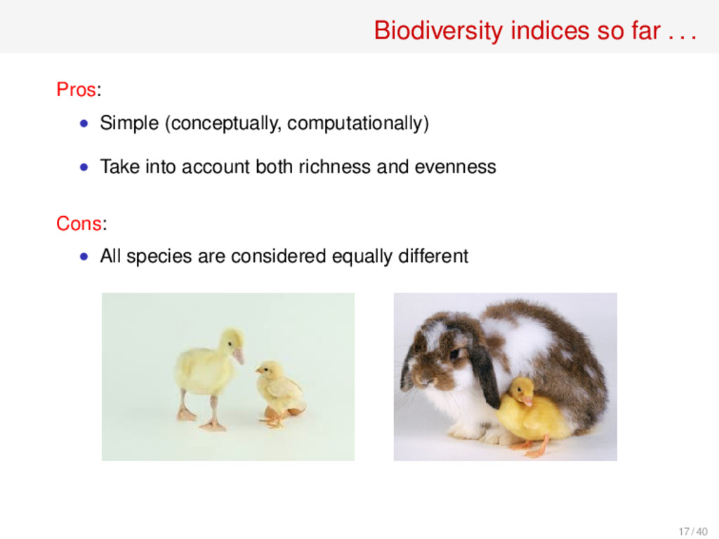
13. Doubling property If we have two independent, non overlapping communities, each with diversity X, and we take the union, the resulting community should have diversity 2X Gini-Simpson indices and Shannon entropy do not satisfy it, but. . . • S satisfies it • 1/IS satisfies it • eH satisfies it 13 / 40
14. Hill’s diversity indices Hill (1973) qD(p) = ∑ i pq i 1 1−q q = 0: 0D(p) = s = S(p) q = 1: 1D(p)(= lim q→1 qD(p)) = ∏i ppi i −1 = eH(p) q = 2: 2D(p) = ∑i p2 i −1 = 1/IS (p) q = ∞: ∞D(p)(= lim q→∞ qD(p)) = max{pi | i = 1,...,s} −1 (Berger-Parker index) ... M. O. Hill, Ecology 5 (1973), 427–432 14 / 40
15. Properties of Hill’s numbers • If p1 = ... = ps, then qD(p) = s for every q 15 / 40
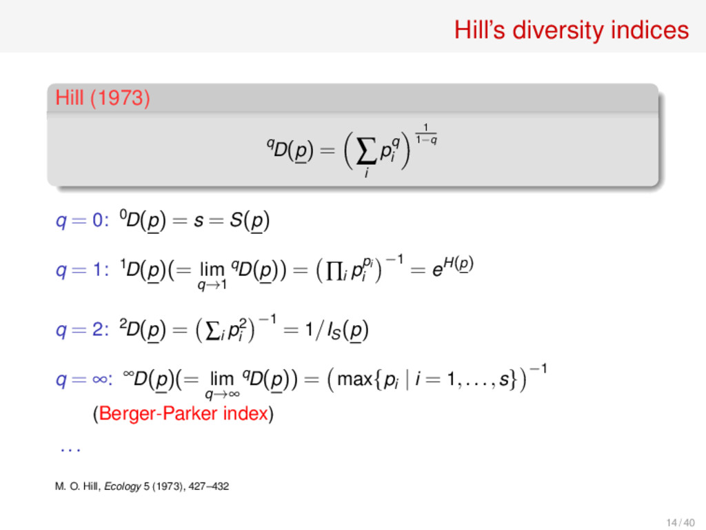
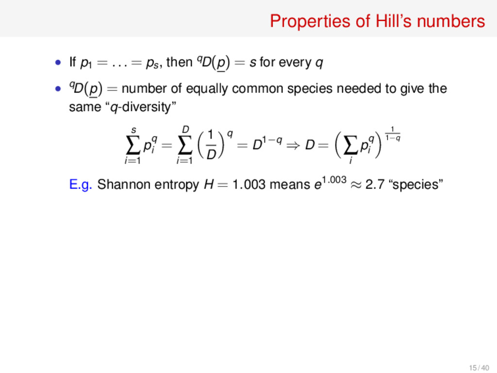
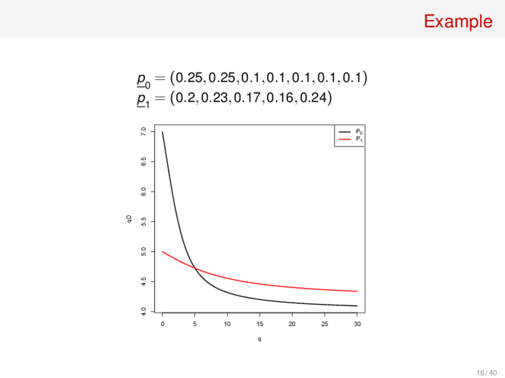
16. Properties of Hill’s numbers • If p1 = ... = ps, then qD(p) = s for every q • qD(p) = number of equally common species needed to give the same “q-diversity” s ∑ i=1 pq i = D ∑ i=1 1 D q = D1−q ⇒ D = ∑ i pq i 1 1−q E.g. Shannon entropy H = 1.003 means e1.003 ≈ 2.7 “species” 15 / 40
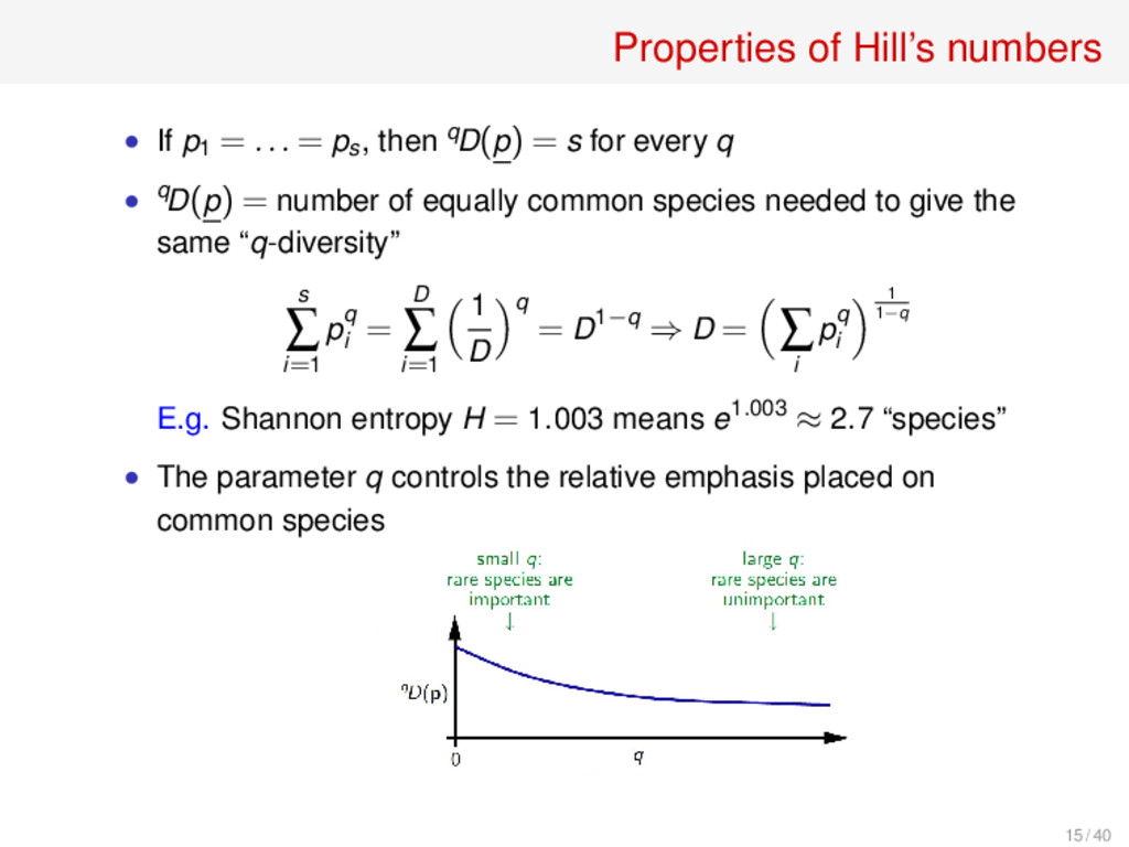
17. Properties of Hill’s numbers • If p1 = ... = ps, then qD(p) = s for every q • qD(p) = number of equally common species needed to give the same “q-diversity” s ∑ i=1 pq i = D ∑ i=1 1 D q = D1−q ⇒ D = ∑ i pq i 1 1−q E.g. Shannon entropy H = 1.003 means e1.003 ≈ 2.7 “species” • The parameter q controls the relative emphasis placed on common species 15 / 40
18. Example p 0 = (0.25,0.25,0.1,0.1,0.1,0.1,0.1) p 1 = (0.2,0.23,0.17,0.16,0.24) 0 5 10 15 20 25 30 4.0 4.5 5.0 5.5 6.0 6.5 7.0 q qD P0 P1 16 / 40
19. Biodiversity indices so far . . . Pros: • Simple (conceptually, computationally) • Take into account both richness and evenness Cons: • All species are considered equally different 17 / 40
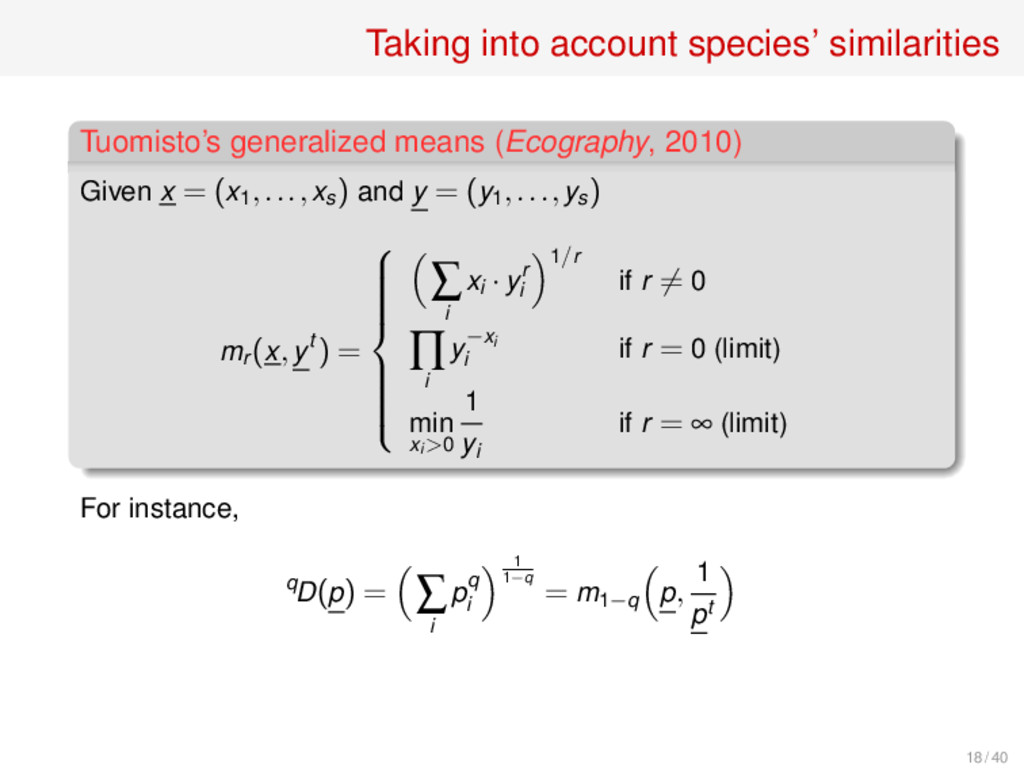
20. Taking into account species’ similarities Tuomisto’s generalized means (Ecography, 2010) Given x = (x1 ,...,xs ) and y = (y1 ,...,ys ) mr (x,yt ) =              ∑ i xi ·yr i 1/r if r = 0 ∏ i y−xi i if r = 0 (limit) min xi >0 1 yi if r = ∞ (limit) For instance, qD(p) = ∑ i pq i 1 1−q = m1−q p, 1 pt 18 / 40
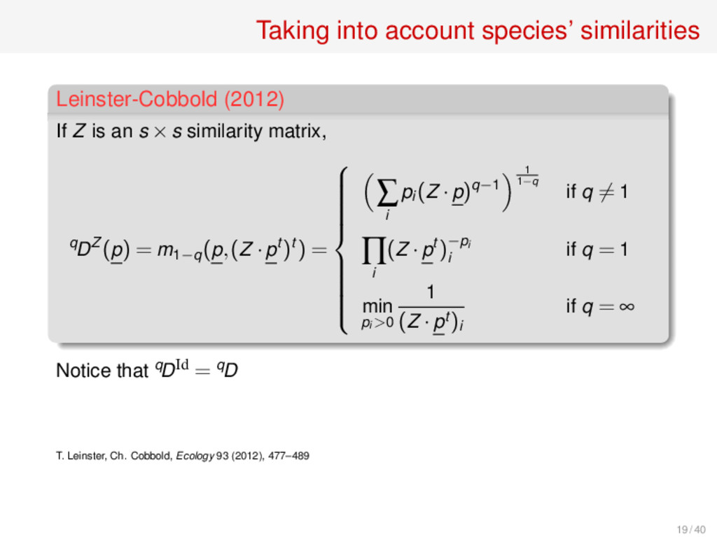
21. Taking into account species’ similarities Leinster-Cobbold (2012) If Z is an s ×s similarity matrix, qDZ (p) = m1−q (p,(Z ·pt )t ) =                  ∑ i pi (Z ·p)q−1 1 1−q if q = 1 ∏ i (Z ·pt )−pi i if q = 1 min pi >0 1 (Z ·pt )i if q = ∞ Notice that qDId = qD T. Leinster, Ch. Cobbold, Ecology 93 (2012), 477–489 19 / 40
22. Taking into account species’ similarities If Z = (zi,j )i,j , qD(p)1−q = ∑ i pi ·pq−1 i qDZ (p)1−q = ∑ i pi · ∑ j zi,j pj q−1 20 / 40
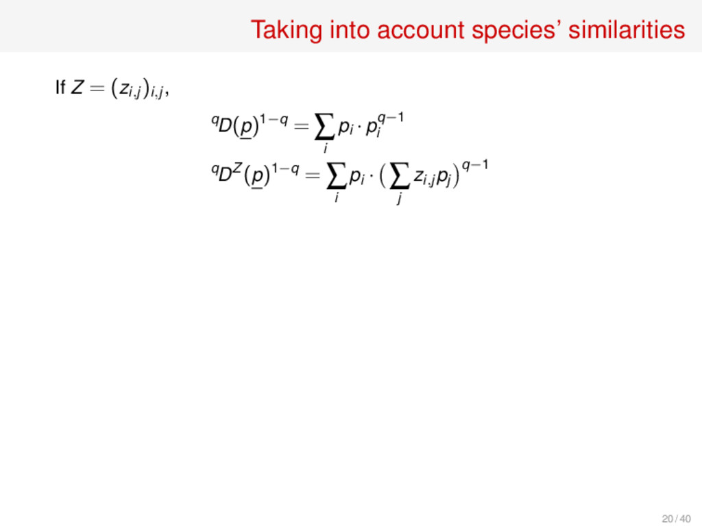
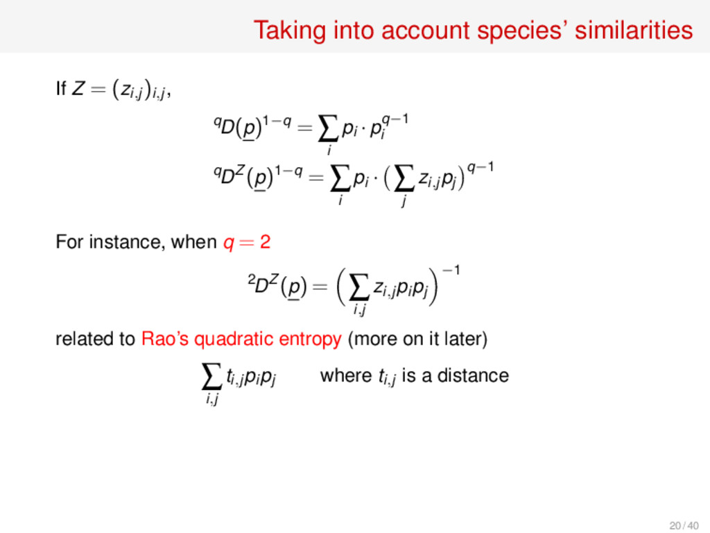
23. Taking into account species’ similarities If Z = (zi,j )i,j , qD(p)1−q = ∑ i pi ·pq−1 i qDZ (p)1−q = ∑ i pi · ∑ j zi,j pj q−1 For instance, when q = 2 2DZ (p) = ∑ i,j zi,j pi pj −1 related to Rao’s quadratic entropy (more on it later) ∑ i,j ti,j pi pj where ti,j is a distance 20 / 40
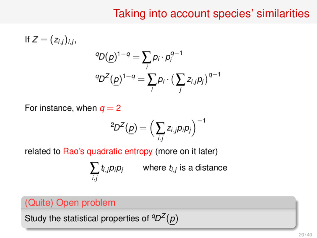
24. Taking into account species’ similarities If Z = (zi,j )i,j , qD(p)1−q = ∑ i pi ·pq−1 i qDZ (p)1−q = ∑ i pi · ∑ j zi,j pj q−1 For instance, when q = 2 2DZ (p) = ∑ i,j zi,j pi pj −1 related to Rao’s quadratic entropy (more on it later) ∑ i,j ti,j pi pj where ti,j is a distance (Quite) Open problem Study the statistical properties of qDZ (p) 20 / 40
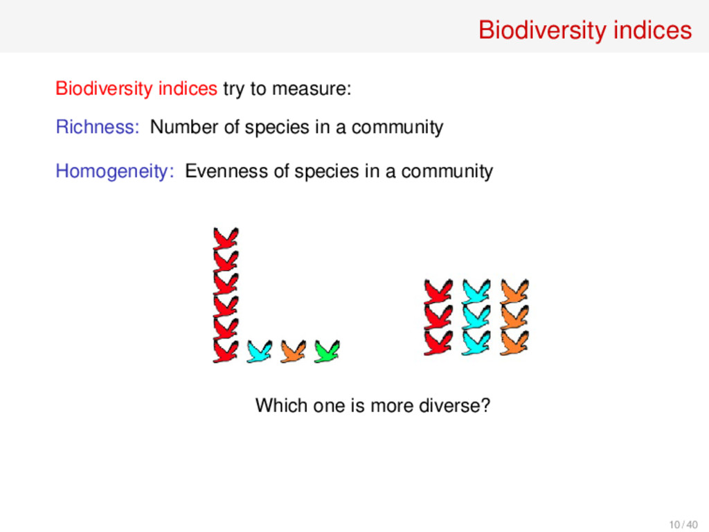
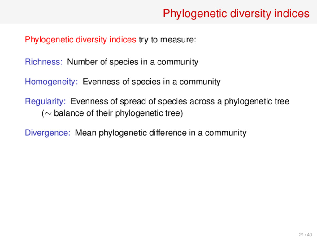
25. Phylogenetic diversity indices Phylogenetic diversity indices try to measure: Richness: Number of species in a community Homogeneity: Evenness of species in a community Regularity: Evenness of spread of species across a phylogenetic tree (∼ balance of their phylogenetic tree) Divergence: Mean phylogenetic difference in a community 21 / 40
26. Measuring phylogenetic diversity • Use phylogenetic or taxonomic similarities in the framework of Hill–Leinster–Cobbold approach • Indices associated to the structure of the phylogenetic tree of a community • Phylogenetic dissimilarities between communities 22 / 40
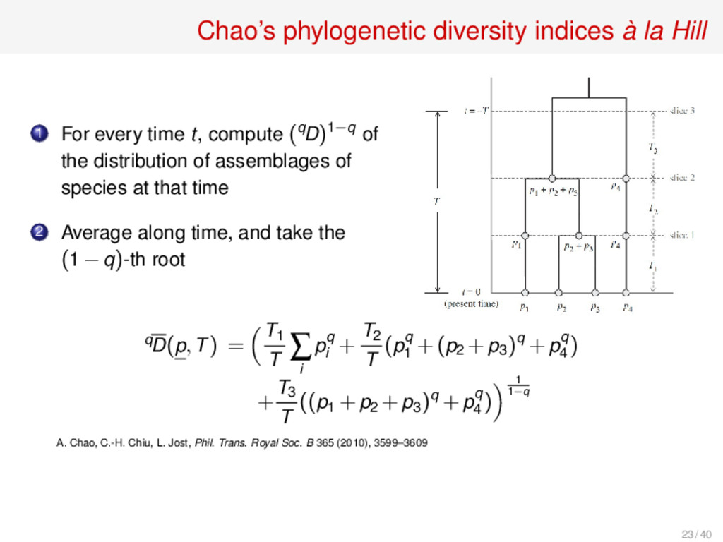
27. Chao’s phylogenetic diversity indices à la Hill 1 For every time t, compute (qD)1−q of the distribution of assemblages of species at that time 2 Average along time, and take the (1 −q)-th root qD(p,T) = T1 T ∑ i pq i + T2 T (pq 1 +(p2 +p3 )q +pq 4 ) + T3 T ((p1 +p2 +p3 )q +pq 4 ) 1 1−q A. Chao, C.-H. Chiu, L. Jost, Phil. Trans. Royal Soc. B 365 (2010), 3599–3609 23 / 40
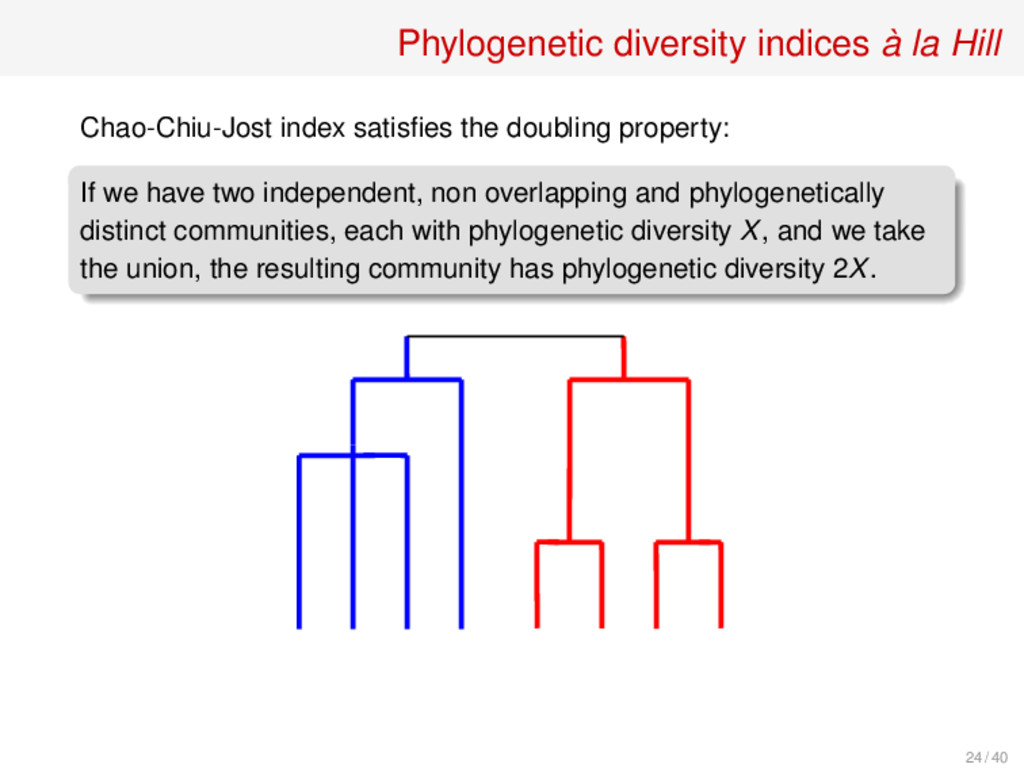
28. Phylogenetic diversity indices à la Hill Chao-Chiu-Jost index satisfies the doubling property: If we have two independent, non overlapping and phylogenetically distinct communities, each with phylogenetic diversity X, and we take the union, the resulting community has phylogenetic diversity 2X. 24 / 40
29. Diversity indices from a phylogenetic tree Phylogenetic diversity Mean depth (distance from the root) of the leaves (Faith, 1992); weighted by species’ abundances (Helmus et al, 2007) 25 / 40
30. Diversity indices from a phylogenetic tree Phylogenetic diversity Mean depth (distance from the root) of the leaves (Faith, 1992); weighted by species’ abundances (Helmus et al, 2007) PD = (3 +3 +2 +1)/4 = 2.25 25 / 40
31. Diversity indices from a phylogenetic tree Phylogenetic diversity Mean depth (distance from the root) of the leaves (Faith, 1992); weighted by species’ abundances (Helmus et al, 2007) WPD = 3 ·0.1 +3 ·0.2 +2 ·0.3 +1 ·0.4 = 1.9 WPD = 3 ·0.4 +3 ·0.3 +2 ·0.2 +1 ·0.1 = 2.6 25 / 40
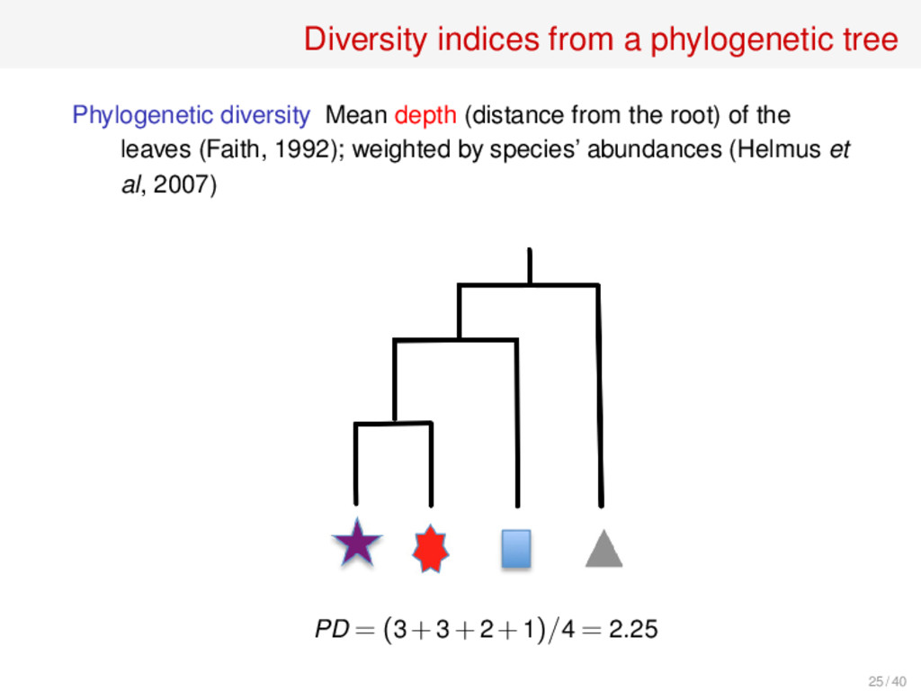
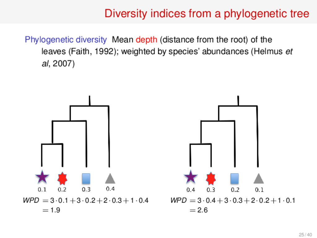
32. Diversity indices from a phylogenetic tree Phylogenetic diversity Mean depth the leaves (Faith, 1992); weighted by species’ abundances (Helmus et al, 2007) Mean phylogenetic distance Mean of the distances between pairs of leaves (Webb, 2000); weighted by species’ abundances (Bell, 2001) Mean nearest neighbour distance Mean of the distances of each leaf to its closest leaf (Webb, 2000); no weighted version Variabilities Variances, instead of means, of the previous values Cophenetic index Mean depth of the least common ancestor of a pair of leaves (UIB, 2013); weighted version in progress 26 such indices compared in S. Pavoine, M. Bonsall, Biol. Rev. 86 (2011), 792–812 26 / 40
33. Abundances vs presence A. Darling et al, PeerJ 2 (2014), e243. 27 / 40
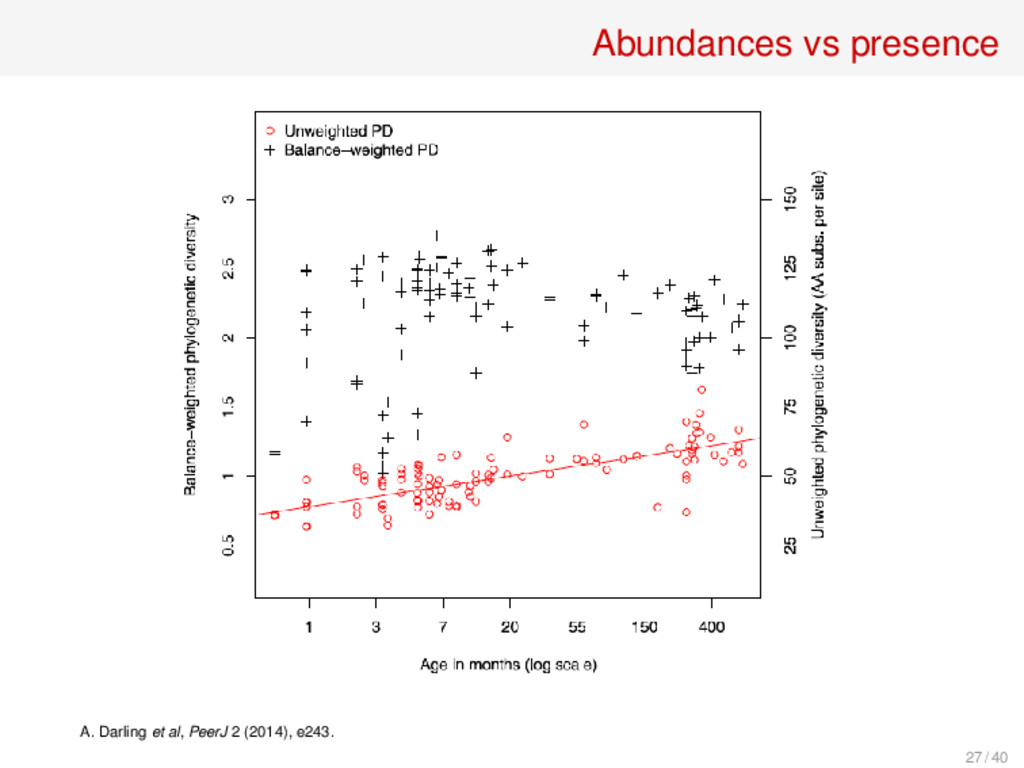
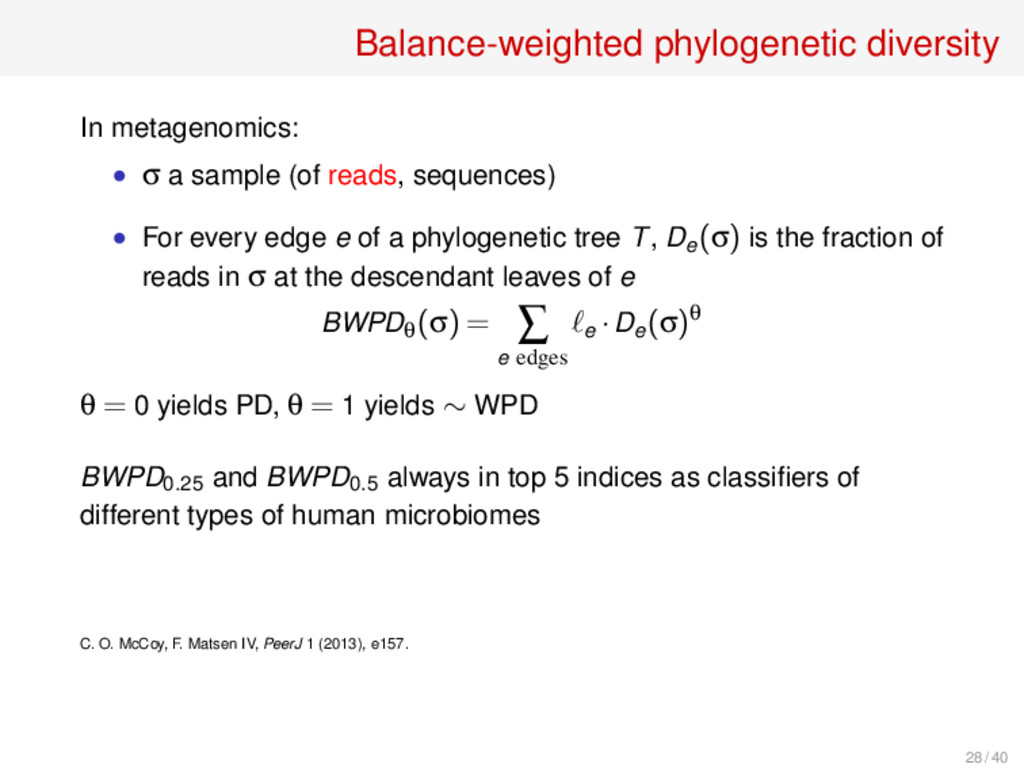
34. Balance-weighted phylogenetic diversity In metagenomics: • σ a sample (of reads, sequences) • For every edge e of a phylogenetic tree T, De (σ) is the fraction of reads in σ at the descendant leaves of e BWPDθ (σ) = ∑ e edges e ·De (σ)θ θ = 0 yields PD, θ = 1 yields ∼ WPD BWPD0.25 and BWPD0.5 always in top 5 indices as classifiers of different types of human microbiomes C. O. McCoy, F. Matsen IV, PeerJ 1 (2013), e157. 28 / 40
35. Classical community comparison Distances between communities based on their (estimated) compositions Rel. abundances p = (p1 ,...,ps ), q = (q1 ,...,qs ) Abs. abundances P = (P1 ,...,Ps ), Q = (Q1 ,...,Qs ) Bray-Curtis index BC = ∑i |pi −qi | 2 or BC = ∑i |Pi −Qi | ∑i (Pi +Qi ) χ2 distance χ2 = ∑ i (pi −qi )2 pi +qi (Weighted) Lr distances . . . . . . 29 / 40
36. Classical community comparison Pros: • Simple (conceptually, computationally) • Take into account both richness and evenness Cons: • All species are considered equally different A déjà vu! 30 / 40
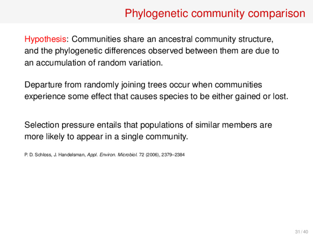
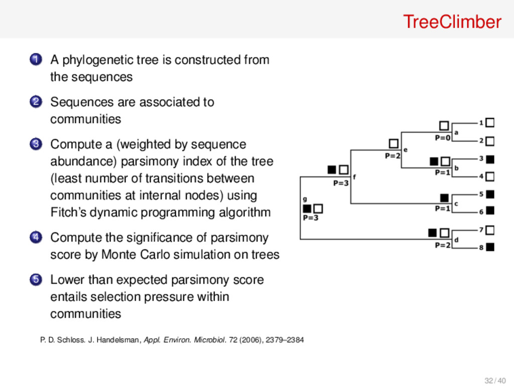
37. Phylogenetic community comparison Hypothesis: Communities share an ancestral community structure, and the phylogenetic differences observed between them are due to an accumulation of random variation. Departure from randomly joining trees occur when communities experience some effect that causes species to be either gained or lost. Selection pressure entails that populations of similar members are more likely to appear in a single community. P. D. Schloss, J. Handelsman, Appl. Environ. Microbiol. 72 (2006), 2379–2384 31 / 40
38. TreeClimber 1 A phylogenetic tree is constructed from the sequences 2 Sequences are associated to communities 3 Compute a (weighted by sequence abundance) parsimony index of the tree (least number of transitions between communities at internal nodes) using Fitch’s dynamic programming algorithm 4 Compute the significance of parsimony score by Monte Carlo simulation on trees 5 Lower than expected parsimony score entails selection pressure within communities P. D. Schloss. J. Handelsman, Appl. Environ. Microbiol. 72 (2006), 2379–2384 32 / 40
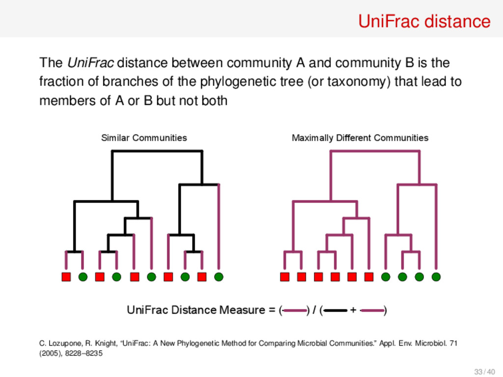
39. UniFrac distance The UniFrac distance between community A and community B is the fraction of branches of the phylogenetic tree (or taxonomy) that lead to members of A or B but not both Similar Communities Maximally Different Communities UniFrac Distance Measure = (------) / (------ + ------) C. Lozupone, R. Knight, “UniFrac: A New Phylogenetic Method for Comparing Microbial Communities.” Appl. Env. Microbiol. 71 (2005), 8228–8235 33 / 40
40. UniFrac distance Significance of UniFrac: Assessed through random relabeling ... # Trees UniFrac Distance Magic level of significance! Randomize Community Labels Observed Tree 34 / 40
41. UniFrac distance Community comparison Pairwise Comparison 0 0 0 0.6 0.5 1.0 0.6 1.0 0.5 UPGMA Distance Matrix Community Tree 35 / 40
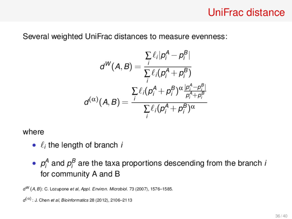
42. UniFrac distance Several weighted UniFrac distances to measure evenness: dW (A,B) = ∑ i i |pA i −pB i | ∑ i i (pA i +pB i ) d(α)(A,B) = ∑ i i (pA i +pB i )α |pA i −pB i | pA i +pB i ∑ i i (pA i +pB i )α where • i the length of branch i • pA i and pB i are the taxa proportions descending from the branch i for community A and B dW (A,B): C. Lozupone et al, Appl. Environ. Microbiol. 73 (2007), 1576–1585. d(α): J. Chen et al, Bioinformatics 28 (2012), 2106–2113 36 / 40
43. Phylogenetic community distances Once you have computed the distances: • PCA, PCoA etc. • Hierarchical clustering • Split networks • Metagenomes are not expected to evolve along a tree • Allows the visualization of incompatible clusters 37 / 40
44. An example Comparison of 16S rRNA time series data from Western English Channel S. Mitra et al, The ISME Journal 4 (2010), 1236-1242 38 / 40
45. An example Comparison of 16S rRNA time series data from Western English Channel S. Mitra et al, The ISME Journal 4 (2010), 1236-1242 39 / 40
46. Final remarks • Many indices measuring ecological richness and homogeneity • Many indices measuring phylogenetic richness and homogeneity • Many indices measuring community composition differences • Several indices measuring community phylogenetic composition differences • I have skipped the spatial component of diversity • No one-size-fits-it-all index in any category • Metagenomics poses its own problems, due to the nature and amount of the data 40 / 40