SOC 4015 & SOC 5050 - Lecture 03

Slides for Lecture 03 of the Saint Louis University Course Quantitative Analysis: Applied Inferential Statistics. These slides cover descriptive statistics and the importance of data visualization.

Transcript

1. You will need GitHub Desktop at the beginning of class. Please make sure you have installed in on your laptop or desktop (it cannot be pre-installed on SLU computers). 
 
 Open it up and log in if you are prompted. Go to Preferences if not prompted (in  menu on macOS or File menu on Windows). WELCOME! GETTING STARTED There is an anonymous entry ticket to complete (link posted in Slack’s #_news channel)
2. DESCRIBING DISTRIBUTIONS QUANTITATIVE ANALYSIS CHRISTOPHER PRENER, PH.D. FALL 2018 WEEK 03 LECTURE 03
3. AGENDA QUANTITATIVE ANALYSIS / WEEK 03 / LECTURE 03 1. Front Matter 2. Getting Organized 3. Visualizing Distributions 4. Describing Distributions 5. Descriptive Stats and Getting Help in R 6. Back Matter
4. ⋆ THEME Today I want to focus on 
 being intentional with how
 we organize work, describe mathematical processes, communicate results, and pose questions.
5. 1 FRONT 
 MATTER
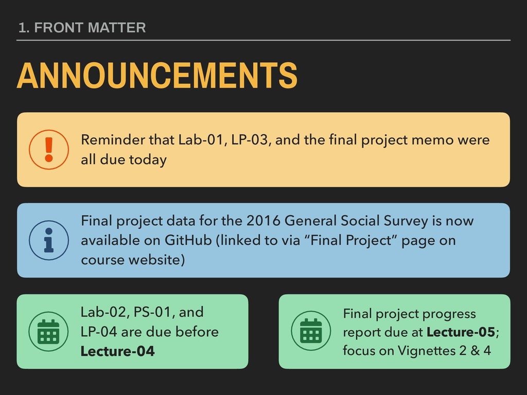
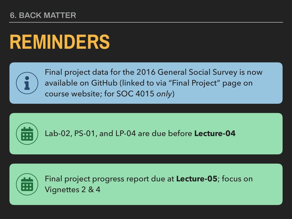
6. Reminder that Lab-01, LP-03, and the final project memo were all due today Lab-02, PS-01, and LP-04 are due before Lecture-04 Final project data for the 2016 General Social Survey is now available on GitHub (linked to via “Final Project” page on course website) 1. FRONT MATTER ANNOUNCEMENTS Final project progress report due at Lecture-05; focus on Vignettes 2 & 4
7. RESOURCES REMINDERS ▸ Course website pages: • Link to specific resources on GitHub • Link to topic index entries that allow you to see all weeks in which specific topics were covered; package index links to documentation • Link to syllabus (and vice versa) ▸ Make sure you’re checking in with the #_news channel on Slack ▸ Post questions in #helpdesk… channels on Slack and celebrate victories in #weekly-wins • Important threads are being catalogued on the lecture webpages 1. FRONT MATTER
8. GETTING ORGANIZED 2
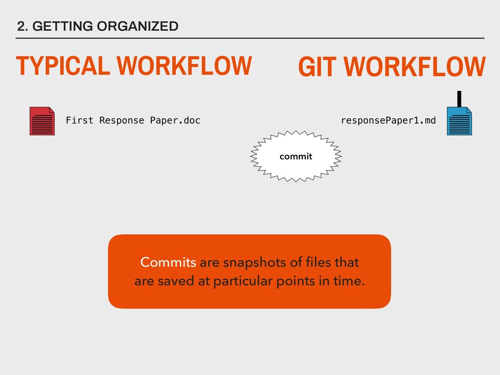
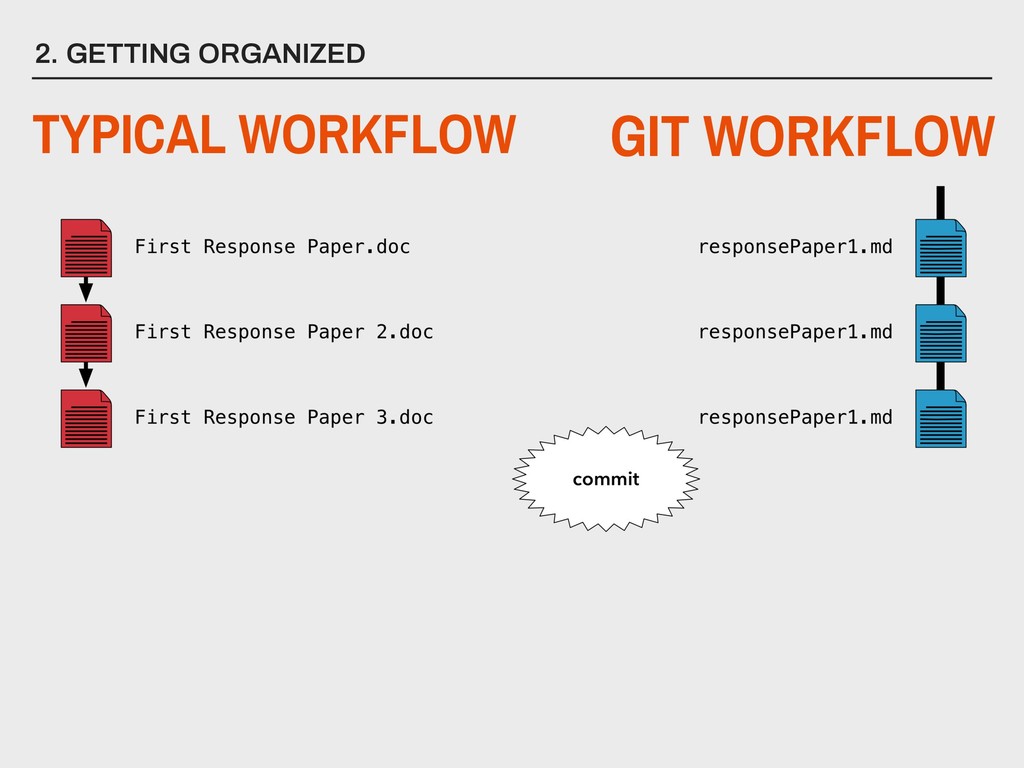
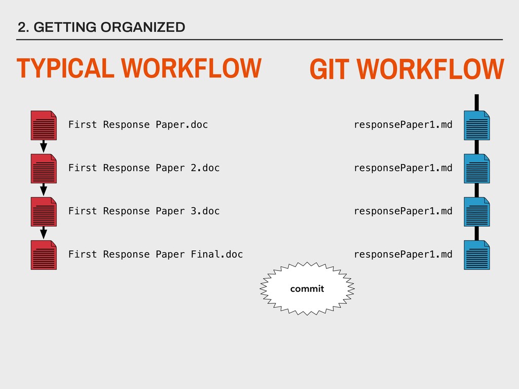
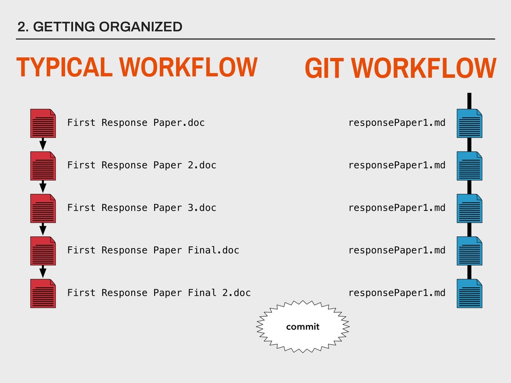
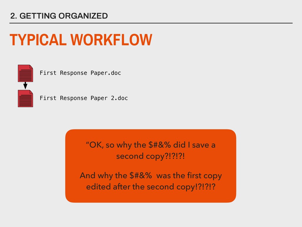
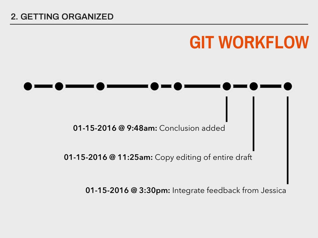
9. KEY QUESTIONS ▸ How do you organize files? ▸ Do you keep different versions of files as your assignment or project progresses? ▸ If you needed your files in 5 years, could you find them? ▸ If you needed your files in 5 years, could you open them? ▸ Do you backup files ever? ▸ If your house was robbed or burned down, would your backup also be destroyed? 2. GETTING ORGANIZED
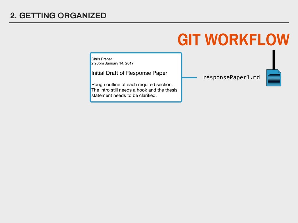
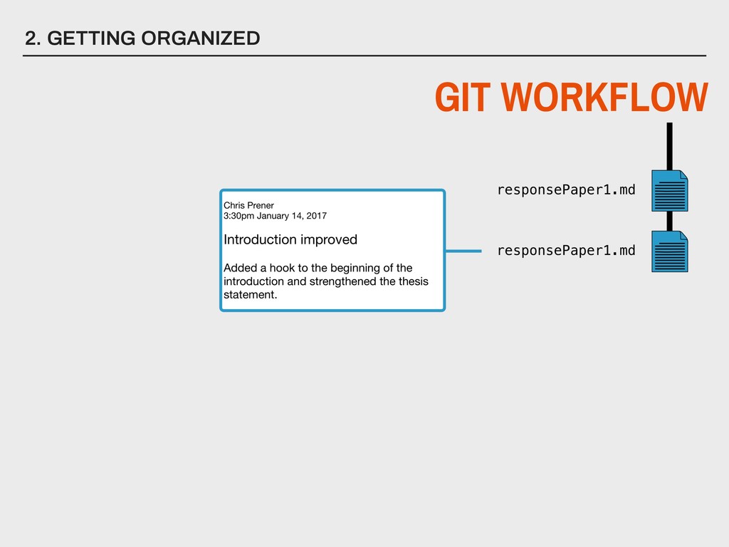
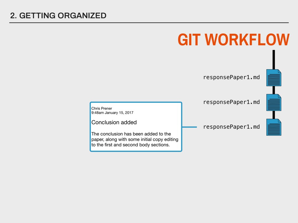
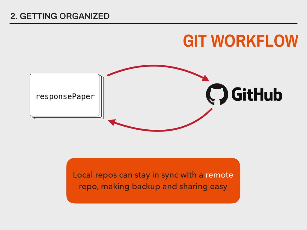
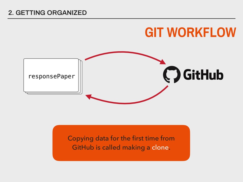
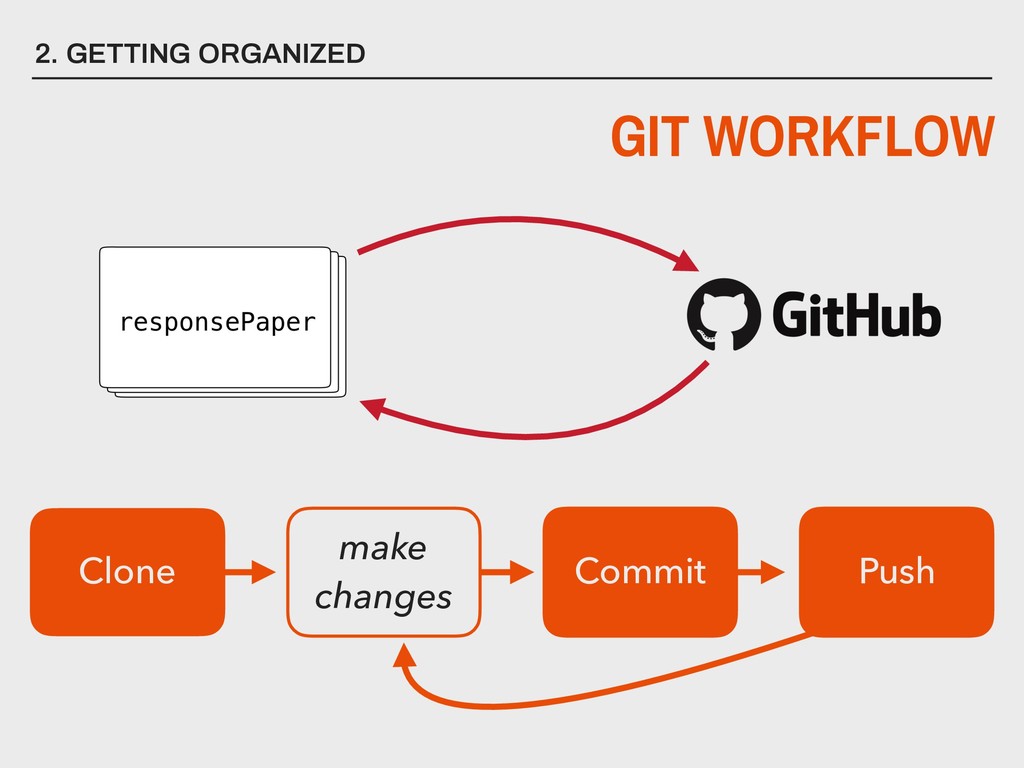
10. KEY QUESTIONS ▸ How do you organize files? ▸ Do you keep different versions of files as your assignment or project progresses? ▸ If you needed your files in 5 years, could you find them? ▸ If you needed your files in 5 years, could you open them? ▸ Do you backup files ever? ▸ If your house was robbed or burned down, would your backup also be destroyed? 2. GETTING ORGANIZED Git & GitHub can help you address all 
 of these key questions/issues!
11. 2. GETTING ORGANIZED GIT BASICS Git is originally a command line tool, and can still be used that way.
12. 2. GETTING ORGANIZED GIT BASICS Top-level directories in Git are called
 repositories. All files placed in a “repo”
 are tracked unless Git is explicitly told
 not to track them.
13. 2. GETTING ORGANIZED TYPICAL WORKFLOW
14. 2. GETTING ORGANIZED TYPICAL WORKFLOW GIT WORKFLOW Commits are snapshots of files that
 are saved at particular points in time.
15. 2. GETTING ORGANIZED TYPICAL WORKFLOW GIT WORKFLOW
16. 2. GETTING ORGANIZED TYPICAL WORKFLOW GIT WORKFLOW
17. 2. GETTING ORGANIZED TYPICAL WORKFLOW GIT WORKFLOW
18. 2. GETTING ORGANIZED TYPICAL WORKFLOW GIT WORKFLOW
19. 2. GETTING ORGANIZED TYPICAL WORKFLOW “OK, so why the $#&% did I save a
 second copy?!?!?! And why the $#&% was the first copy 
 edited after the second copy!?!?!?
20. 2. GETTING ORGANIZED GIT WORKFLOW
21. 2. GETTING ORGANIZED GIT WORKFLOW
22. 2. GETTING ORGANIZED GIT WORKFLOW
23. 2. GETTING ORGANIZED GIT WORKFLOW
24. 2. GETTING ORGANIZED GIT WORKFLOW Local repos can stay in sync with a remote repo, making backup and sharing easy
25. 2. GETTING ORGANIZED GIT WORKFLOW Copying data for the first time from 
 GitHub is called making a clone.
26. 2. GETTING ORGANIZED GIT WORKFLOW Clone make
 changes Commit Push
27. VISUALIZING DISTRIBUTIONS 3
28. WHAT IS A DISTRIBUTION?
29. WHAT IS A DISTRIBUTION?
30. WHAT IS A DISTRIBUTION?
31. 3. VISUALIZING DISTRIBUTIONS OUR WORKFLOW 1. Plan 2. Organize 3. Document 4. Execute For Each
 Step:
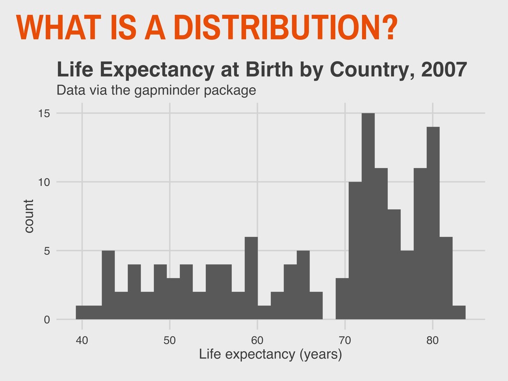
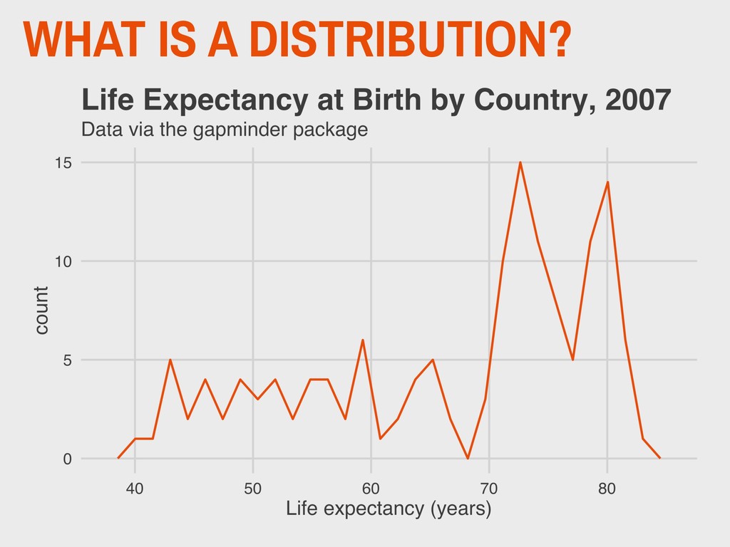
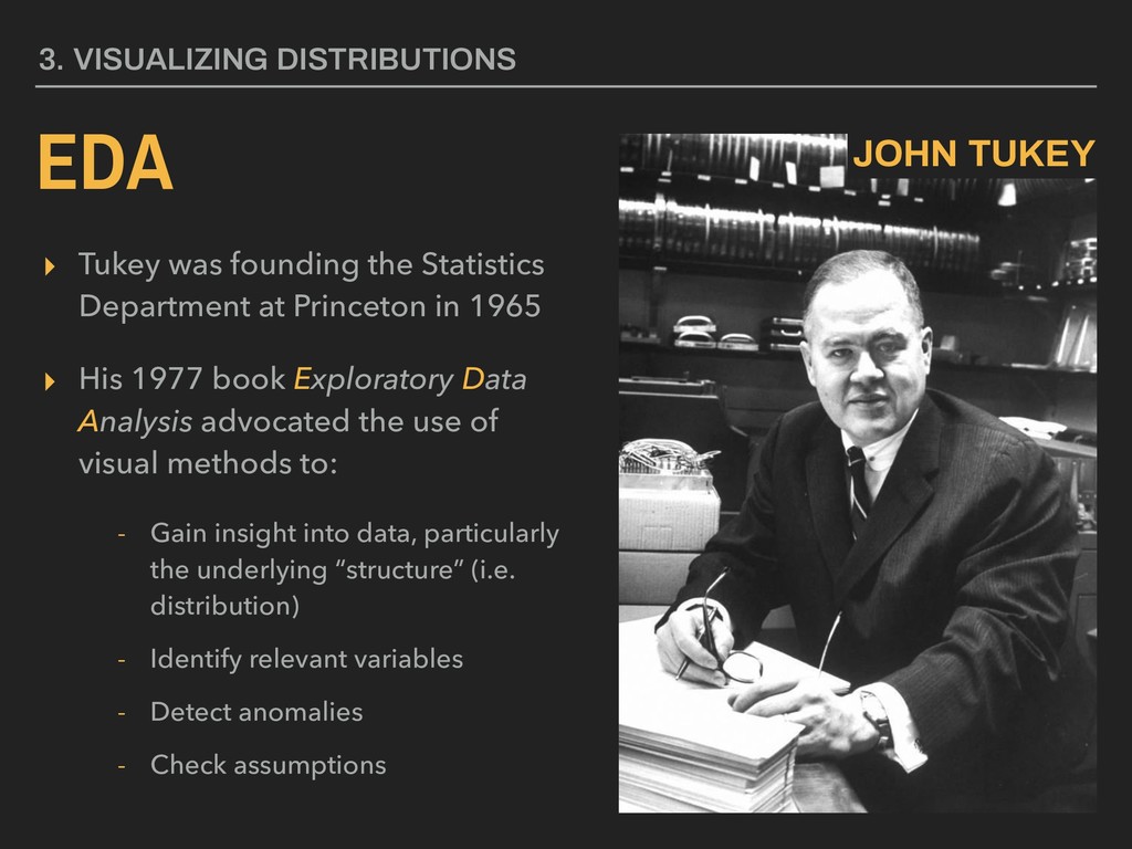
32. ▸ Tukey was founding the Statistics Department at Princeton in 1965 ▸ His 1977 book Exploratory Data Analysis advocated the use of visual methods to: - Gain insight into data, particularly the underlying “structure” (i.e. distribution) - Identify relevant variables - Detect anomalies - Check assumptions 3. VISUALIZING DISTRIBUTIONS EDA JOHN TUKEY
33. PLOTTING DISTRIBUTIONS geom_histogram() geom_freqpoly() geom_density() geom_bar()
34. PLOTTING DISTRIBUTIONS geom_histogram() geom_freqpoly() geom_density() geom_bar()
35. DESCRIBING DISTRIBUTIONS 4
36. WHAT IS A MODEL? “REAL” WORLD
37. WHAT IS A MODEL? APPROXIMATION OF “REAL” WORLD
38. COMPARING MODELS “REAL” WORLD GOOD FIT POOR FIT
39. SOME DATA
40. A STATISTICAL MODEL
41. A SECOND STATISTICAL MODEL
42. COMPARING MODELS “REAL” WORLD POOR FIT GOOD FIT
43. 4. DESCRIBING DISTRIBUTIONS DESCRIPTIVE STATISTICS Central Tendency
 How values “congregate”
 around the center of the distribution Dispersion
 The “spread” of the 
 values in a distribution
44. 4. DESCRIBING DISTRIBUTIONS DESCRIPTIVE STATISTICS Central Tendency
 How values “congregate”
 around the center of the distribution Mode Mean Median
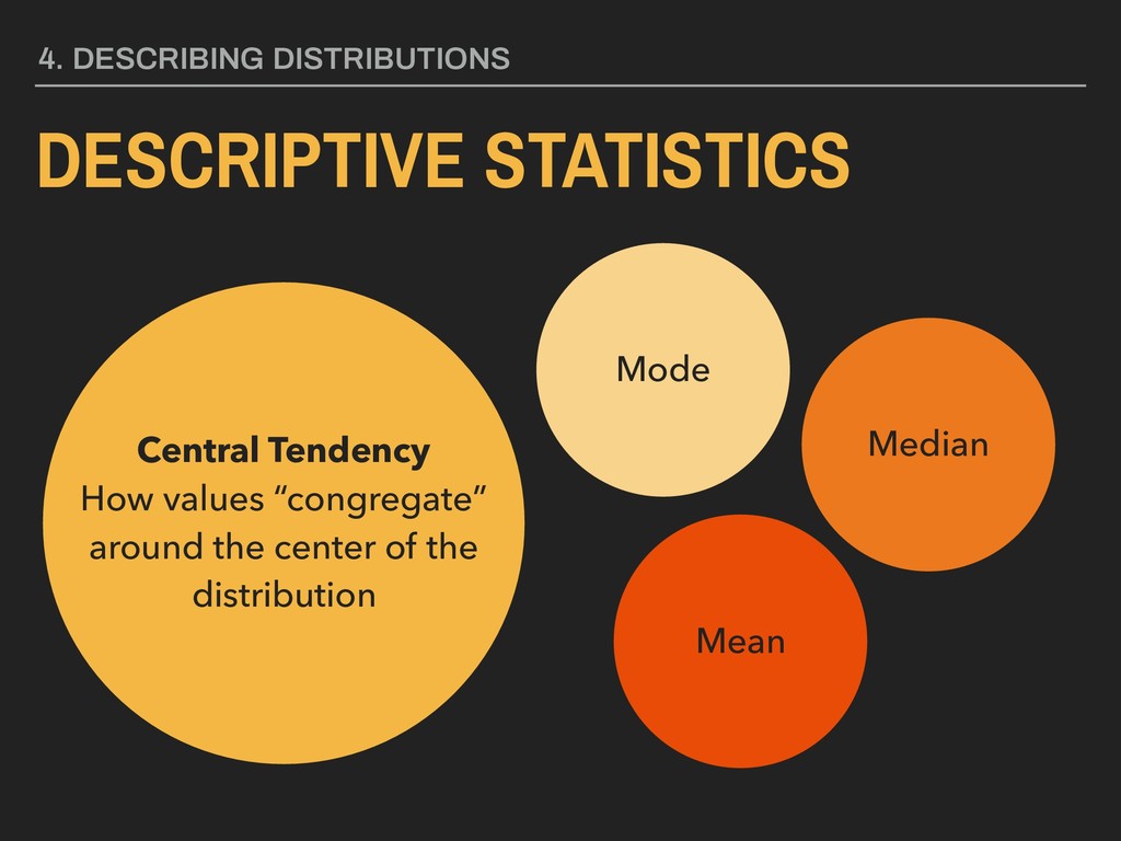
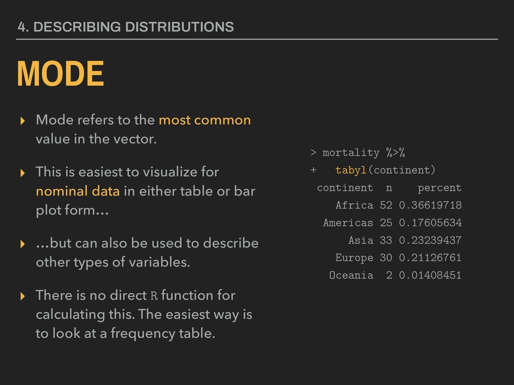
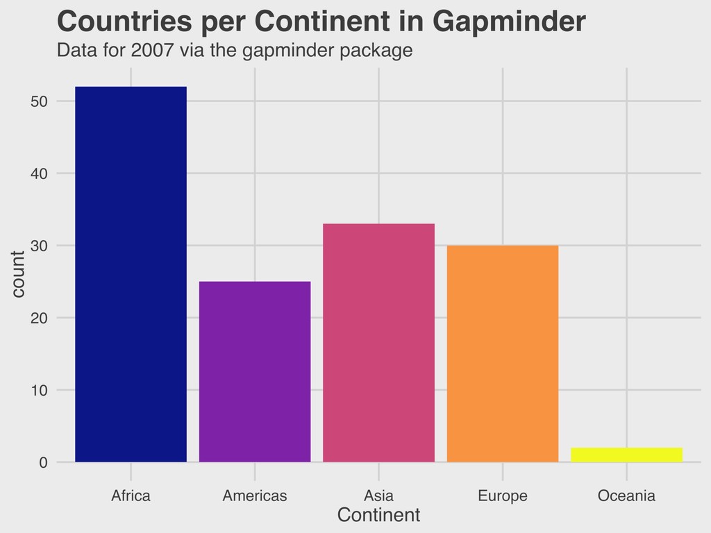
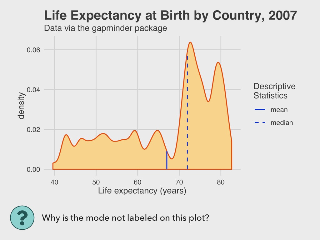
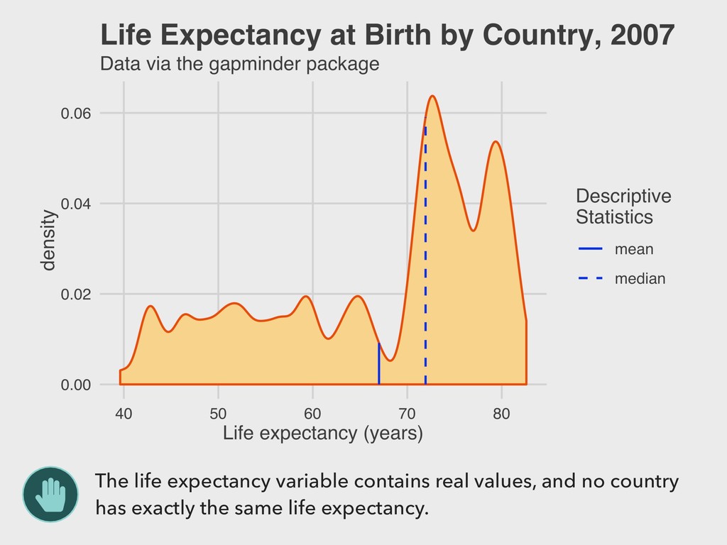
45. ▸ Mode refers to the most common value in the vector. ▸ This is easiest to visualize for nominal data in either table or bar plot form… ▸ …but can also be used to describe other types of variables. ▸ There is no direct R function for calculating this. The easiest way is to look at a frequency table. 4. DESCRIBING DISTRIBUTIONS MODE > mortality %>% + tabyl(continent) continent n percent Africa 52 0.36619718 Americas 25 0.17605634 Asia 33 0.23239437 Europe 30 0.21126761 Oceania 2 0.01408451
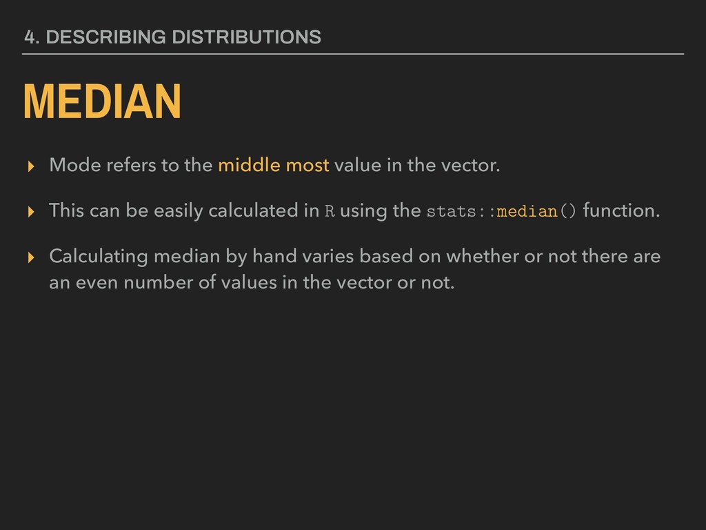
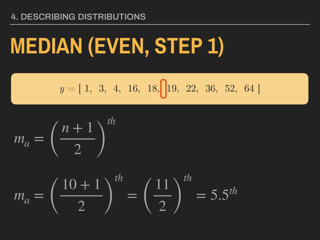
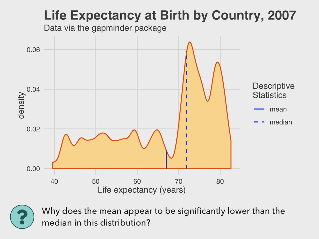
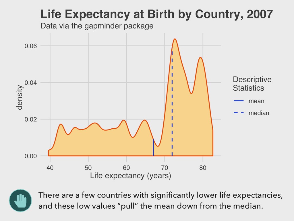
49. MEDIAN ▸ Mode refers to the middle most value in the vector. ▸ This can be easily calculated in R using the stats::median() function. ▸ Calculating median by hand varies based on whether or not there are an even number of values in the vector or not. 4. DESCRIBING DISTRIBUTIONS
50. ▸ m = the median item's term ▸ n = the number of items in the given vector 4. DESCRIBING DISTRIBUTIONS Let: MEDIAN (ODD) m = ( n + 1 2 ) th
51. 4. DESCRIBING DISTRIBUTIONS MEDIAN (ODD) x = [ 1, 3, 4, 16, 18, 19, 22, 36, 52, 64, 81 ] m = ( n + 1 2 ) th m = ( 11 + 1 2 ) th = ( 12 2 ) th = 6th
52. ▸ ma = the middlemost position in the vector ▸ n = the number of items in the given vector 4. DESCRIBING DISTRIBUTIONS Let: MEDIAN (EVEN, STEP 1) ma = ( n + 1 2 ) th
53. 4. DESCRIBING DISTRIBUTIONS MEDIAN (EVEN, STEP 1) y = [ 1, 3, 4, 16, 18, 19, 22, 36, 52, 64 ] ma = ( n + 1 2 ) th ma = ( 10 + 1 2 ) th = ( 11 2 ) th = 5.5th
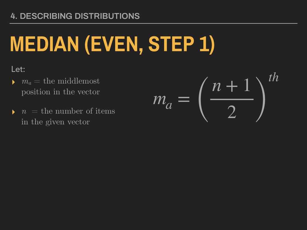
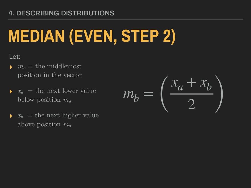
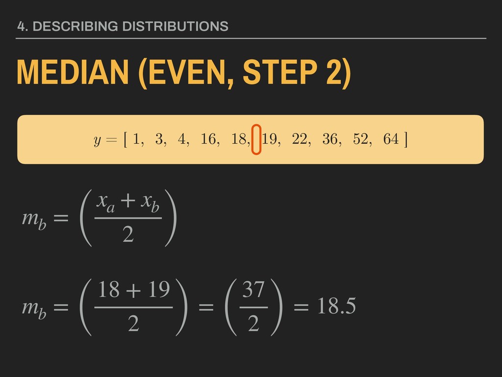
54. ▸ ma = the middlemost position in the vector ▸ xa = the next lower value below position ma ▸ xb = the next higher value above position ma 4. DESCRIBING DISTRIBUTIONS Let: MEDIAN (EVEN, STEP 2) mb = ( xa + xb 2 )
55. 4. DESCRIBING DISTRIBUTIONS MEDIAN (EVEN, STEP 2) y = [ 1, 3, 4, 16, 18, 19, 22, 36, 52, 64 ] mb = ( xa + xb 2 ) mb = ( 18 + 19 2 ) = ( 37 2 ) = 18.5
56. MEAN ▸ Mean refers to the average value in the vector. ▸ This can be easily calculated in R using the stats::mean() function. ▸ Calculating mean by hand involves the use of sigma or summation notation
 ▸ Greek letter (“mu”) used for referring to the population mean, which is often theoretical, meaning we cannot directly measure it ▸ The mean is the first moment of a distribution 4. DESCRIBING DISTRIBUTIONS
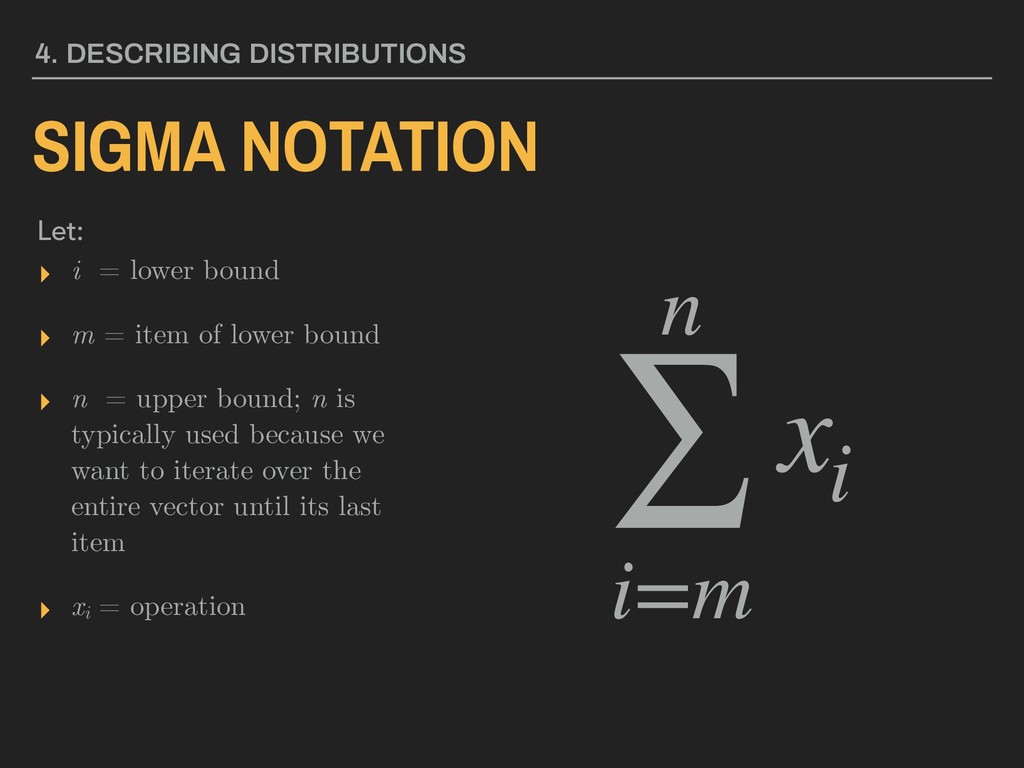
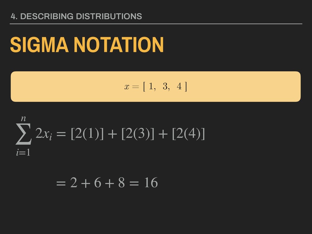
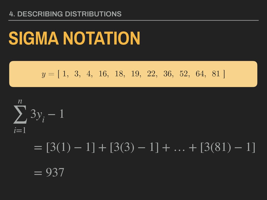
57. ▸ i = lower bound ▸ m = item of lower bound ▸ n = upper bound; n is typically used because we want to iterate over the entire vector until its last item ▸ xi = operation 4. DESCRIBING DISTRIBUTIONS Let: SIGMA NOTATION n ∑ i=m xi
58. 4. DESCRIBING DISTRIBUTIONS SIGMA NOTATION x = [ 1, 3, 4 ] n ∑ i=1 2xi = [2(1)] + [2(3)] + [2(4)] = 2 + 6 + 8 = 16
59. 4. DESCRIBING DISTRIBUTIONS SIGMA NOTATION y = [ 1, 3, 4, 16, 18, 19, 22, 36, 52, 64, 81 ] n ∑ i=1 3y i − 1 = [3(1) − 1] + [3(3) − 1] + … + [3(81) − 1] = 937
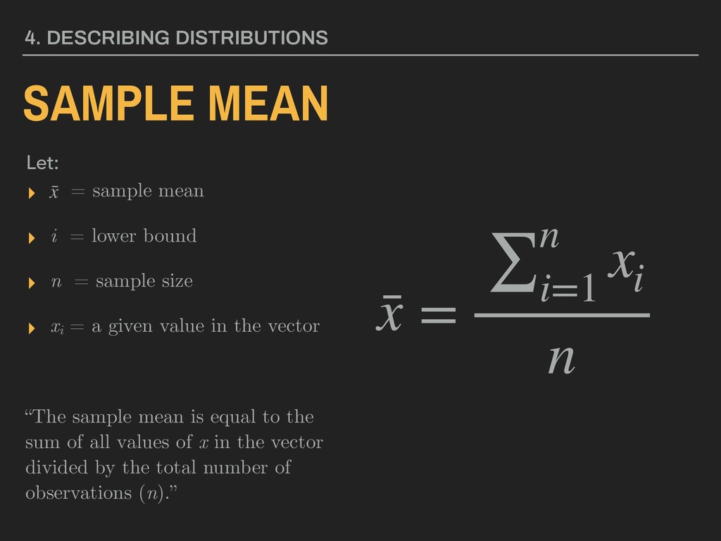
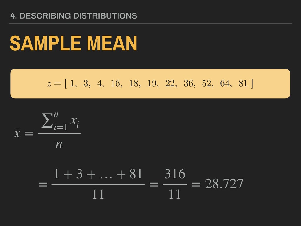
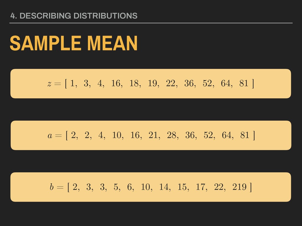
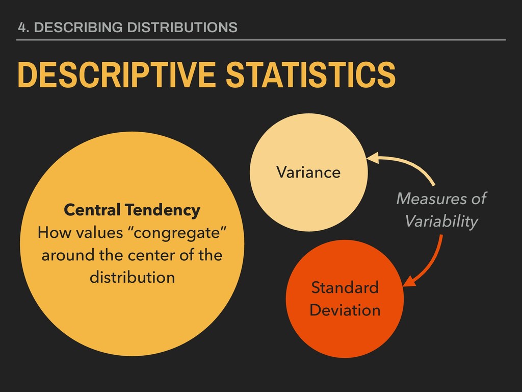
60. ▸ = sample mean ▸ i = lower bound ▸ n = sample size ▸ xi = a given value in the vector “The sample mean is equal to the sum of all values of x in the vector divided by the total number of observations (n).” 4. DESCRIBING DISTRIBUTIONS Let: SAMPLE MEAN ¯ x = ∑n i=1 xi n ¯ x
61. 4. DESCRIBING DISTRIBUTIONS SAMPLE MEAN z = [ 1, 3, 4, 16, 18, 19, 22, 36, 52, 64, 81 ] ¯ x = ∑n i=1 xi n = 1 + 3 + … + 81 11 = 316 11 = 28.727
62. 4. DESCRIBING DISTRIBUTIONS SAMPLE MEAN z = [ 1, 3, 4, 16, 18, 19, 22, 36, 52, 64, 81 ] a = [ 2, 2, 4, 10, 16, 21, 28, 36, 52, 64, 81 ] b = [ 2, 3, 3, 5, 6, 10, 14, 15, 17, 22, 219 ]
67. ? Why does the mean appear to be significantly lower than the median in this distribution?
68. There are a few countries with significantly lower life expectancies, and these low values “pull” the mean down from the median.
69. ? Why is the mode not labeled on this plot?
70. The life expectancy variable contains real values, and no country has exactly the same life expectancy.
71. 4. DESCRIBING DISTRIBUTIONS DESCRIPTIVE STATISTICS Central Tendency
 How values “congregate”
 around the center of the distribution Variance Standard
 Deviation Measures of 
 Variability
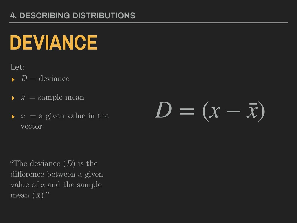
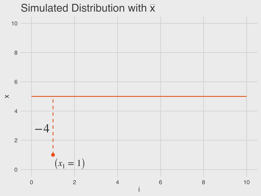
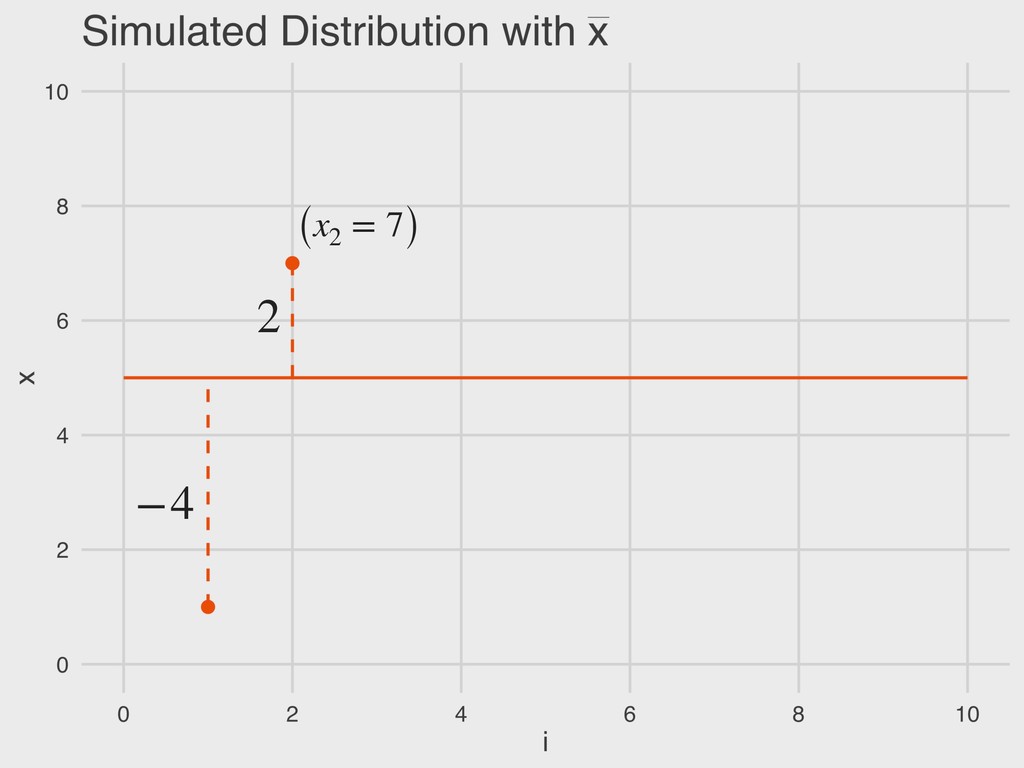
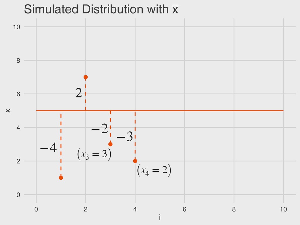
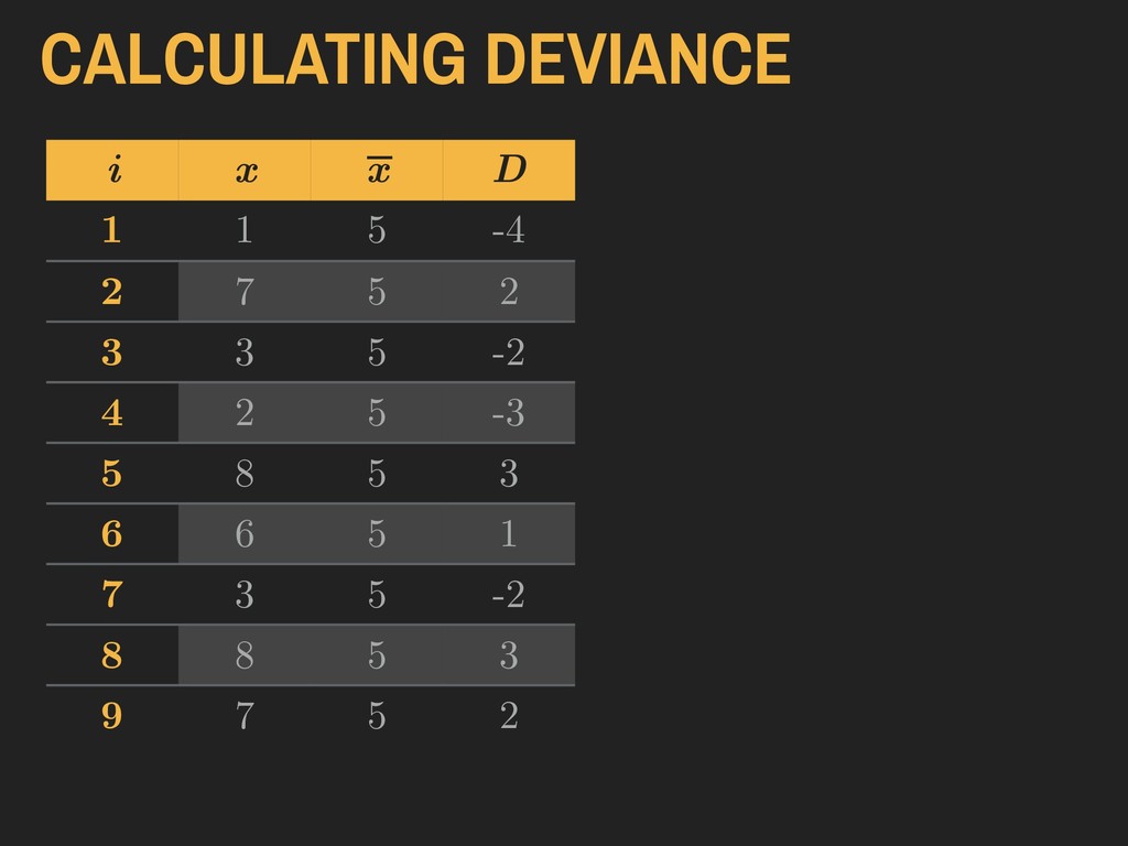
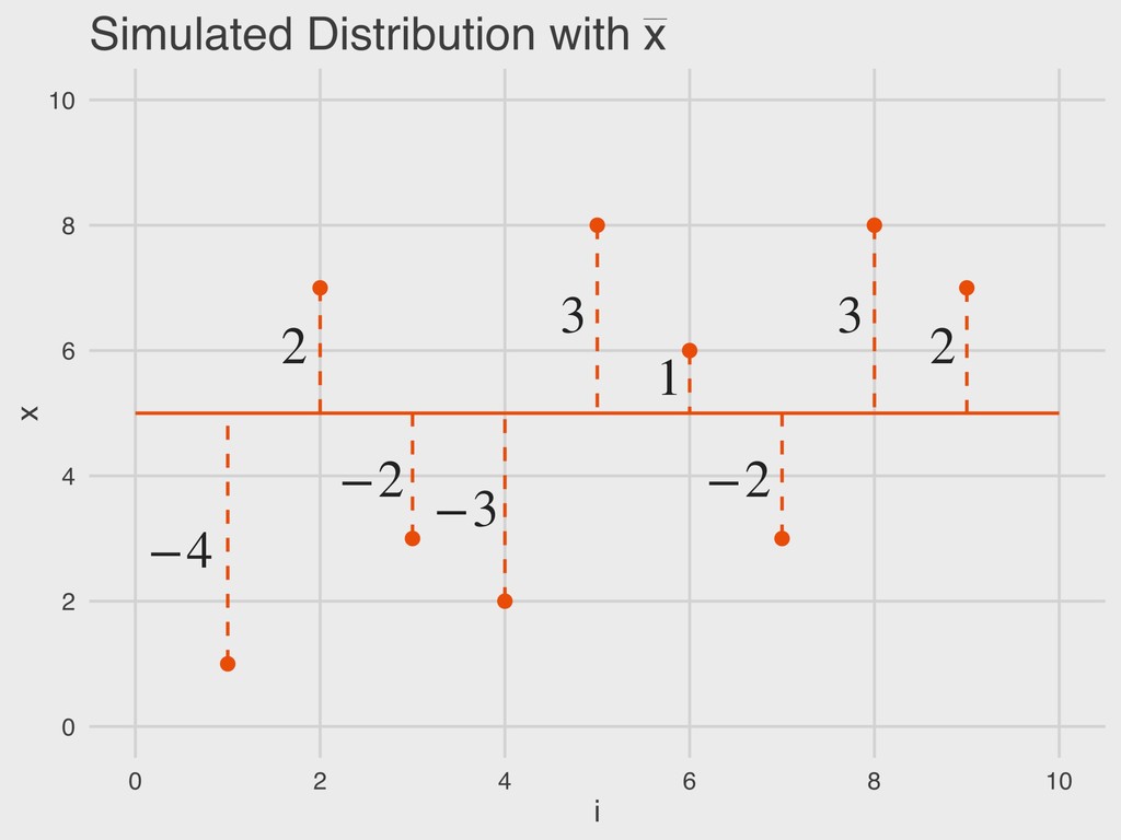
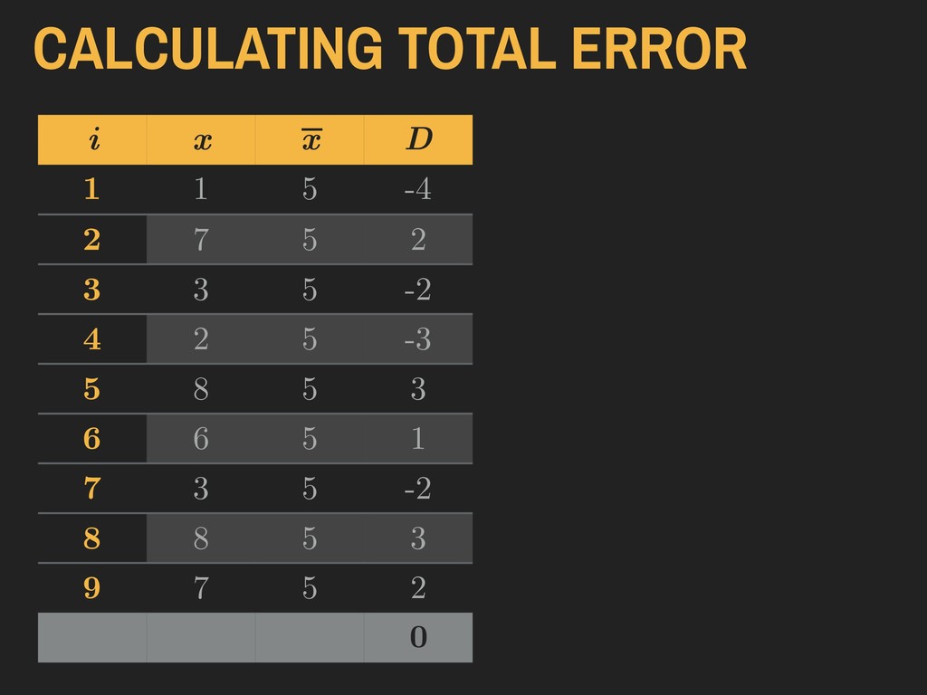
72. ▸ D = deviance ▸ = sample mean ▸ x = a given value in the vector “The deviance (D) is the difference between a given value of x and the sample mean ( ).” 4. DESCRIBING DISTRIBUTIONS Let: DEVIANCE D = (x − ¯ x) ¯ x ¯ x
73. ¯ x
74. −4 (x1 = 1)
75. −4 (x2 = 7) 2
76. −4 (x4 = 2) 2 (x3 = 3) −2 −3
77. −4 2 −2 −3 3 1 3 −2 2
78. CALCULATING DEVIANCE i x x D 1 1 5 -4 2 7 5 2 3 3 5 -2 4 2 5 -3 5 8 5 3 6 6 5 1 7 3 5 -2 8 8 5 3 9 7 5 2 0 ̅
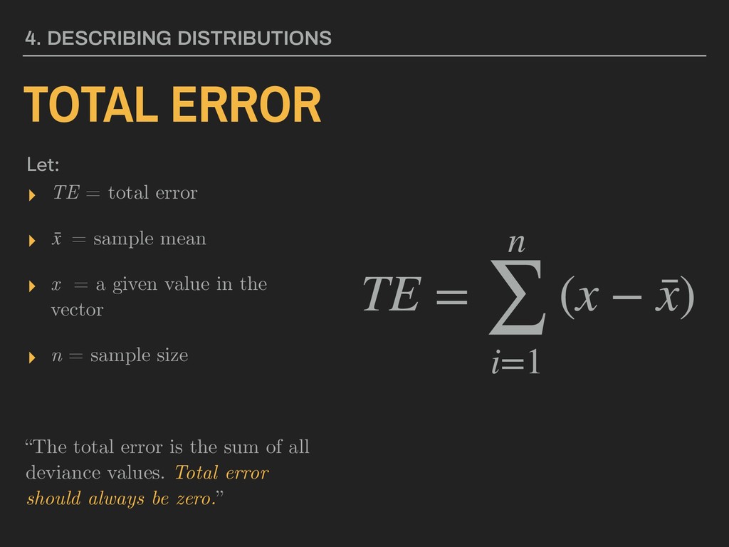
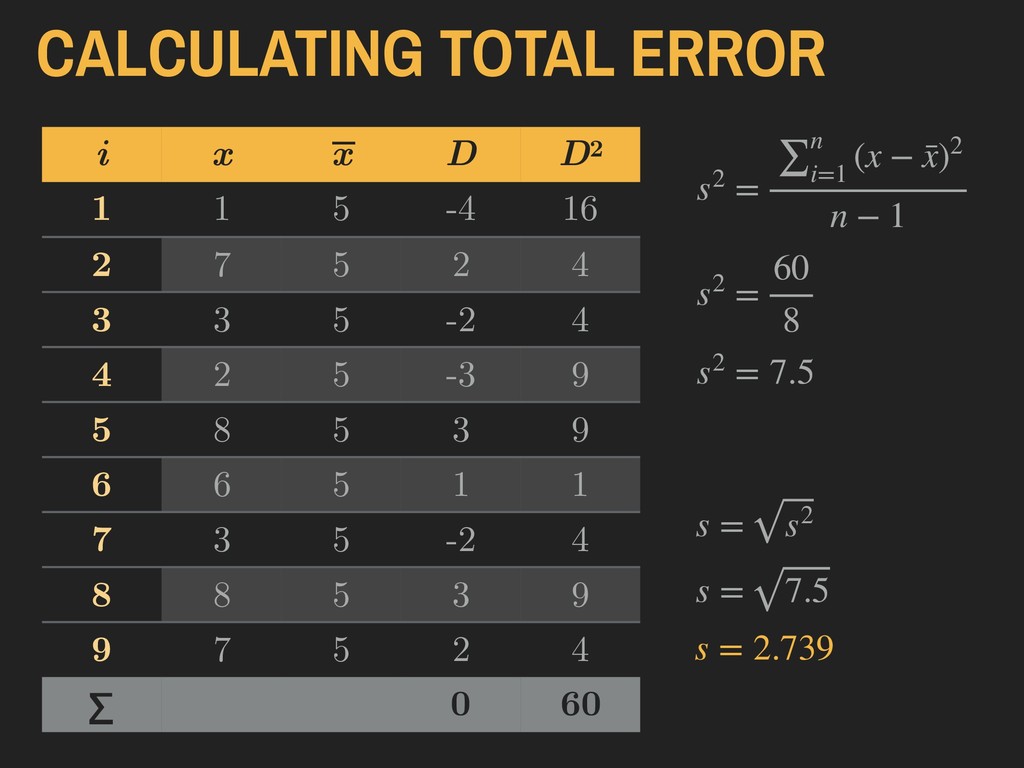
79. ▸ TE = total error ▸ = sample mean ▸ x = a given value in the vector ▸ n = sample size “The total error is the sum of all deviance values. Total error should always be zero.” 4. DESCRIBING DISTRIBUTIONS Let: TOTAL ERROR TE = n ∑ i=1 (x − ¯ x) ¯ x
80. −4 2 −2 −3 3 1 3 −2 2
81. CALCULATING TOTAL ERROR i x x D 1 1 5 -4 2 7 5 2 3 3 5 -2 4 2 5 -3 5 8 5 3 6 6 5 1 7 3 5 -2 8 8 5 3 9 7 5 2 0 ̅
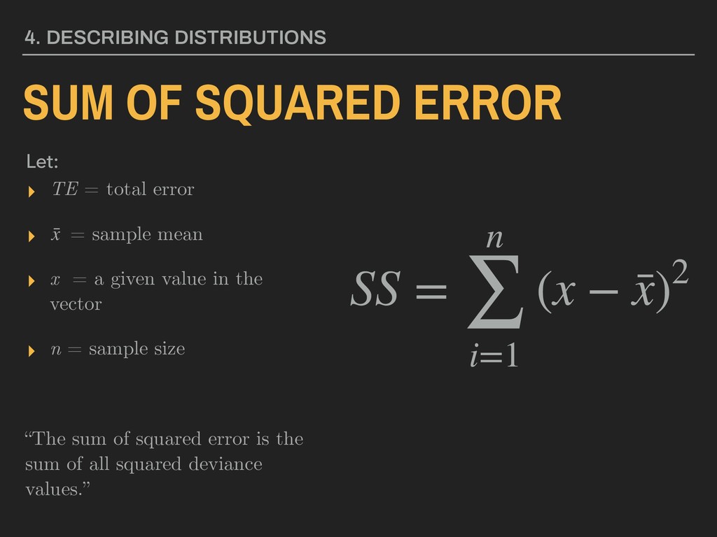
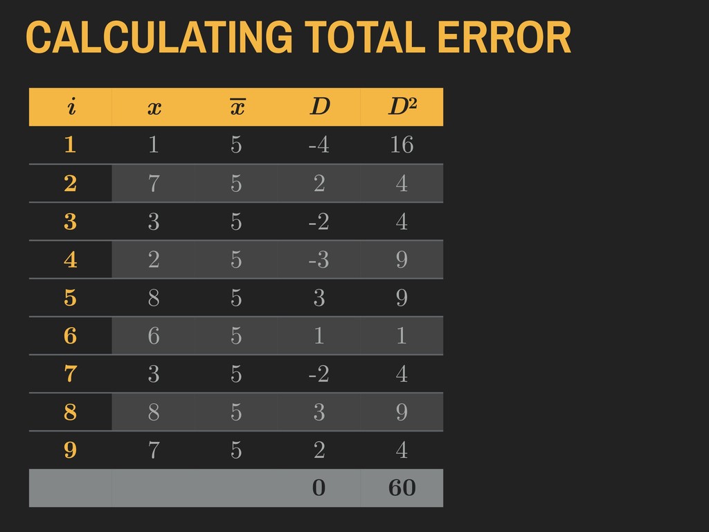
82. ▸ TE = total error ▸ = sample mean ▸ x = a given value in the vector ▸ n = sample size “The sum of squared error is the sum of all squared deviance values.” 4. DESCRIBING DISTRIBUTIONS Let: SUM OF SQUARED ERROR SS = n ∑ i=1 (x − ¯ x)2 ¯ x
83. CALCULATING TOTAL ERROR i x x D D2 1 1 5 -4 16 2 7 5 2 4 3 3 5 -2 4 4 2 5 -3 9 5 8 5 3 9 6 6 5 1 1 7 3 5 -2 4 8 8 5 3 9 9 7 5 2 4 0 60 ̅
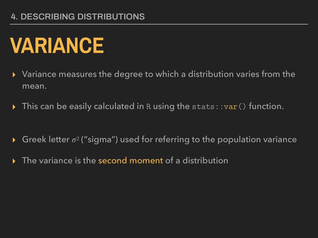
84. VARIANCE ▸ Variance measures the degree to which a distribution varies from the mean. ▸ This can be easily calculated in R using the stats::var() function.
 ▸ Greek letter 2 (“sigma”) used for referring to the population variance ▸ The variance is the second moment of a distribution 4. DESCRIBING DISTRIBUTIONS
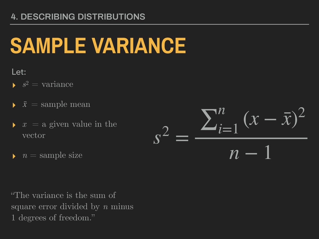
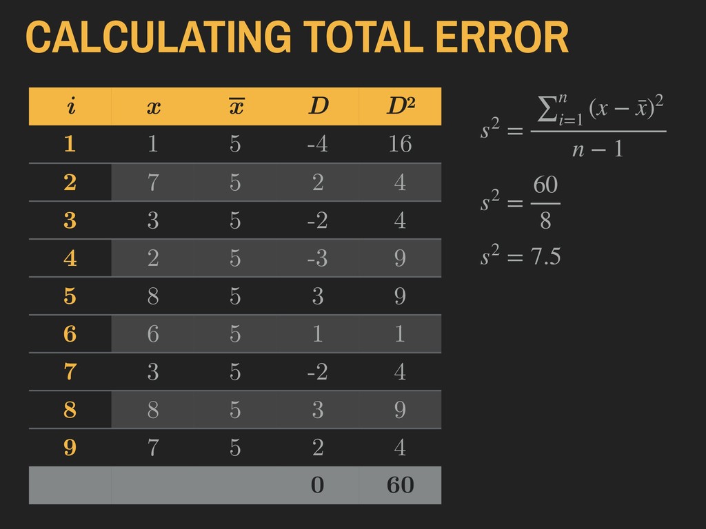
85. ▸ s2 = variance ▸ = sample mean ▸ x = a given value in the vector ▸ n = sample size “The variance is the sum of square error divided by n minus 1 degrees of freedom.” 4. DESCRIBING DISTRIBUTIONS Let: SAMPLE VARIANCE s2 = ∑n i=1 (x − ¯ x)2 n − 1 ¯ x
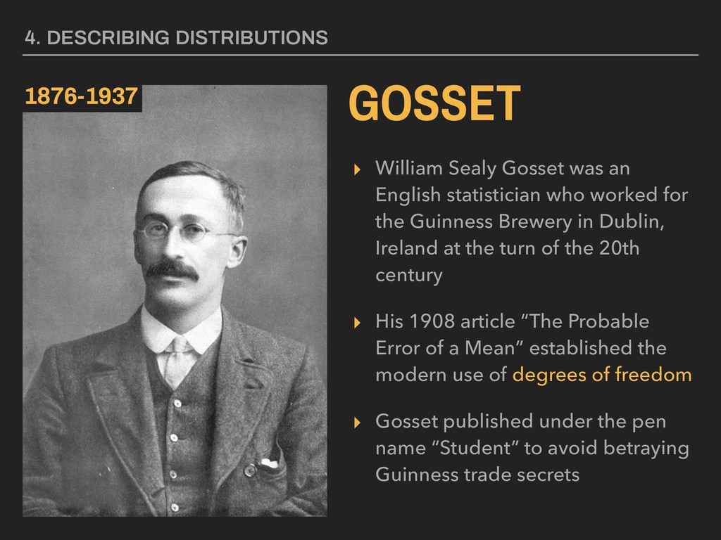
86. ▸ William Sealy Gosset was an English statistician who worked for the Guinness Brewery in Dublin, Ireland at the turn of the 20th century ▸ His 1908 article “The Probable Error of a Mean” established the modern use of degrees of freedom ▸ Gosset published under the pen name “Student” to avoid betraying Guinness trade secrets 4. DESCRIBING DISTRIBUTIONS GOSSET 1876-1937
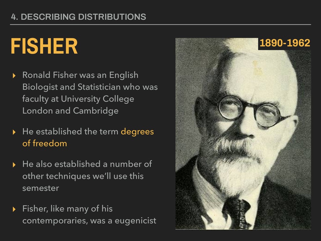
87. ▸ Ronald Fisher was an English Biologist and Statistician who was faculty at University College London and Cambridge ▸ He established the term degrees of freedom ▸ He also established a number of other techniques we’ll use this semester ▸ Fisher, like many of his contemporaries, was a eugenicist 4. DESCRIBING DISTRIBUTIONS FISHER 1890-1962
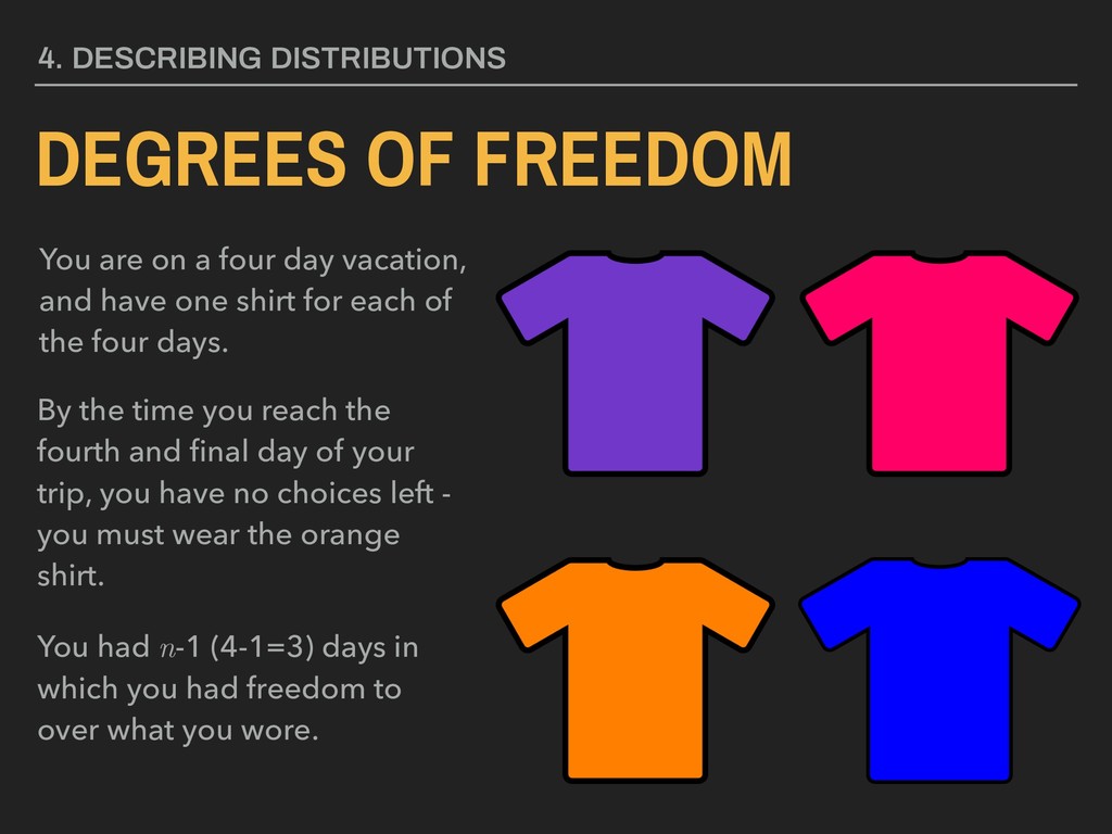
88. 4. DESCRIBING DISTRIBUTIONS DEGREES OF FREEDOM You are on a four day vacation, and have one shirt for each of the four days. By the time you reach the fourth and final day of your trip, you have no choices left - you must wear the orange shirt. You had n-1 (4-1=3) days in which you had freedom to over what you wore.
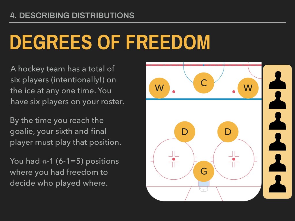
89. 4. DESCRIBING DISTRIBUTIONS DEGREES OF FREEDOM A hockey team has a total of six players (intentionally!) on the ice at any one time. You have six players on your roster. By the time you reach the goalie, your sixth and final player must play that position. You had n-1 (6-1=5) positions where you had freedom to decide who played where. C W W D D G
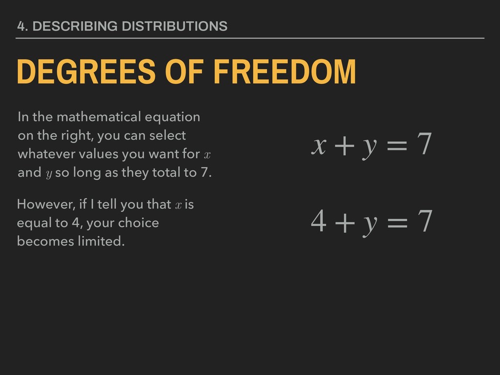
90. 4. DESCRIBING DISTRIBUTIONS DEGREES OF FREEDOM In the mathematical equation on the right, you can select whatever values you want for x and y so long as they total to 7. However, if I tell you that x is equal to 4, your choice becomes limited. x + y = 7 4 + y = 7
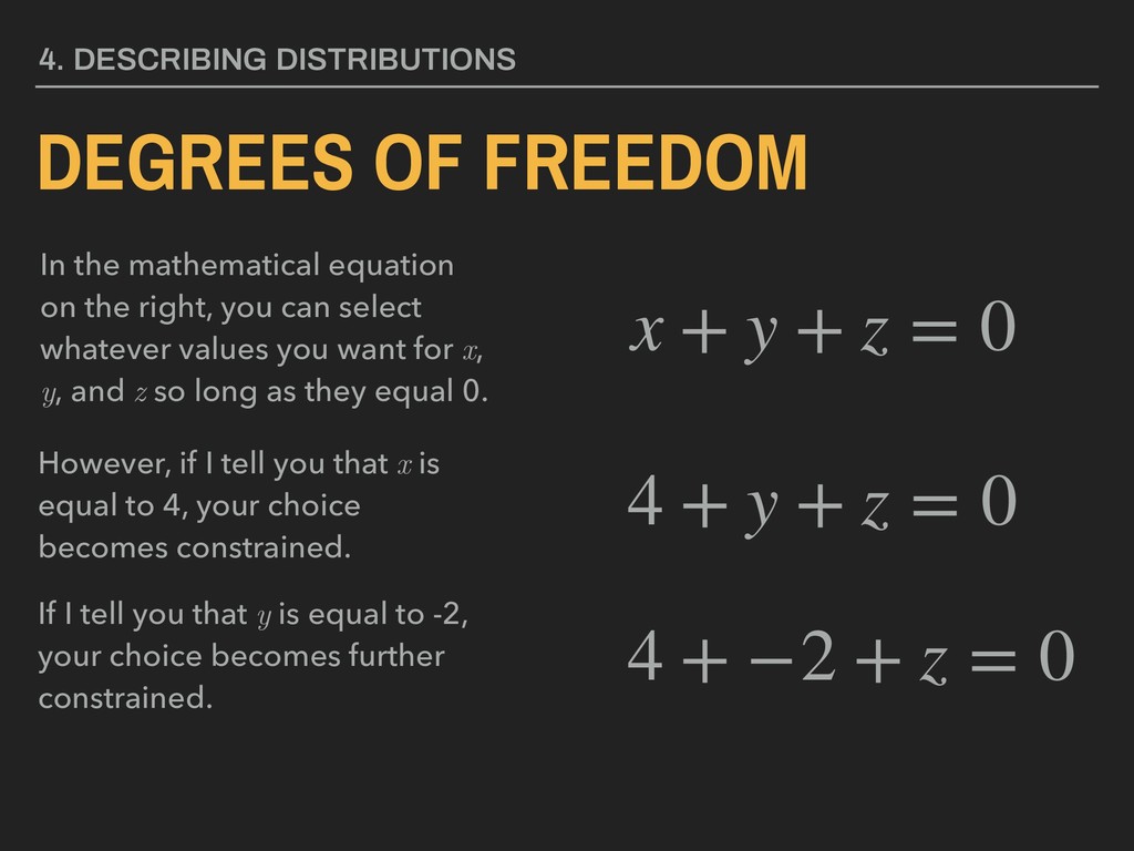
91. 4. DESCRIBING DISTRIBUTIONS DEGREES OF FREEDOM In the mathematical equation on the right, you can select whatever values you want for x, y, and z so long as they equal 0. However, if I tell you that x is equal to 4, your choice becomes constrained. If I tell you that y is equal to -2, your choice becomes further constrained. x + y + z = 0 4 + y + z = 0 4 + −2 + z = 0
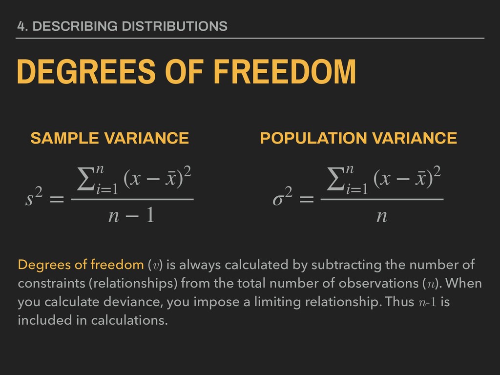
92. 4. DESCRIBING DISTRIBUTIONS DEGREES OF FREEDOM s2 = ∑n i=1 (x − ¯ x)2 n − 1 σ2 = ∑n i=1 (x − ¯ x)2 n Degrees of freedom (v) is always calculated by subtracting the number of constraints (relationships) from the total number of observations (n). When you calculate deviance, you impose a limiting relationship. Thus n-1 is included in calculations. SAMPLE VARIANCE POPULATION VARIANCE
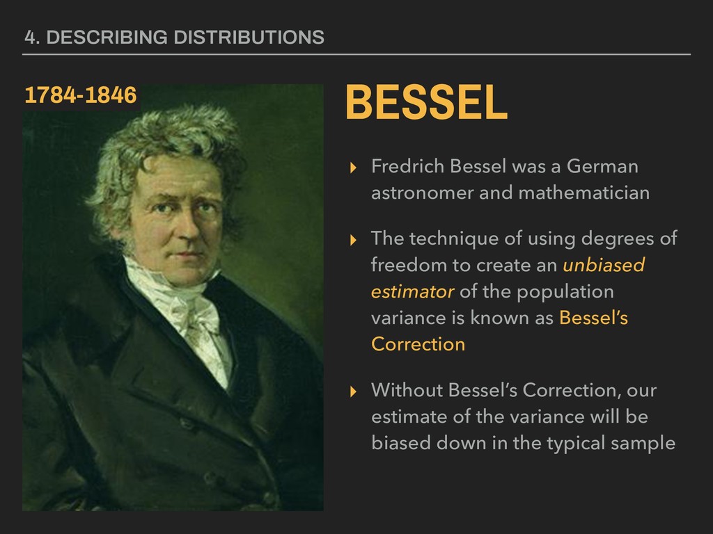
93. ▸ Fredrich Bessel was a German astronomer and mathematician ▸ The technique of using degrees of freedom to create an unbiased estimator of the population variance is known as Bessel’s Correction ▸ Without Bessel’s Correction, our estimate of the variance will be biased down in the typical sample 4. DESCRIBING DISTRIBUTIONS BESSEL 1784-1846
94. CALCULATING TOTAL ERROR i x x D D2 1 1 5 -4 16 2 7 5 2 4 3 3 5 -2 4 4 2 5 -3 9 5 8 5 3 9 6 6 5 1 1 7 3 5 -2 4 8 8 5 3 9 9 7 5 2 4 0 60 ̅ s2 = ∑n i=1 (x − ¯ x)2 n − 1 s2 = 60 8 s2 = 7.5
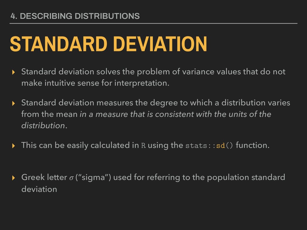
95. STANDARD DEVIATION ▸ Standard deviation solves the problem of variance values that do not make intuitive sense for interpretation. ▸ Standard deviation measures the degree to which a distribution varies from the mean in a measure that is consistent with the units of the distribution. ▸ This can be easily calculated in R using the stats::sd() function.
 ▸ Greek letter (“sigma”) used for referring to the population standard deviation 4. DESCRIBING DISTRIBUTIONS
96. ▸ s = standard deviation ▸ = sample mean ▸ x = a given value in the vector ▸ n = sample size “The standard deviation is the square root of the variance.” 4. DESCRIBING DISTRIBUTIONS Let: STANDARD DEVIATION s = ∑n i=1 (x − ¯ x)2 n − 1 ¯ x
97. CALCULATING TOTAL ERROR i x x D D2 1 1 5 -4 16 2 7 5 2 4 3 3 5 -2 4 4 2 5 -3 9 5 8 5 3 9 6 6 5 1 1 7 3 5 -2 4 8 8 5 3 9 9 7 5 2 4 ∑ 0 60 ̅ s2 = ∑n i=1 (x − ¯ x)2 n − 1 s2 = 60 8 s2 = 7.5 s = s2 s = 7.5 s = 2.739
98. 4. DESCRIBING DISTRIBUTIONS DESCRIPTIVE STATISTICS Central Tendency
 How values “congregate”
 around the center of the distribution Dispersion
 The “spread” of the 
 values in a distribution
99. 4. DESCRIBING DISTRIBUTIONS DESCRIPTIVE STATISTICS Dispersion
 The “spread” of the 
 values in a distribution Inter-quartile Range Range
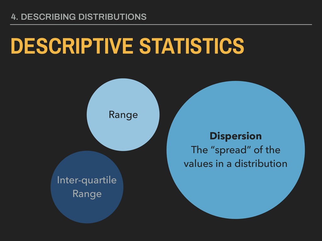
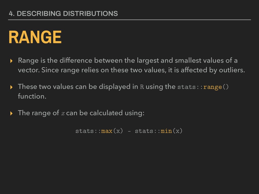
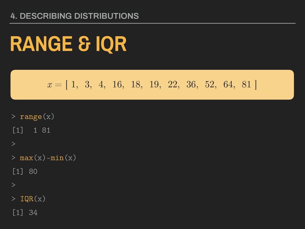
100. RANGE ▸ Range is the difference between the largest and smallest values of a vector. Since range relies on these two values, it is affected by outliers. ▸ These two values can be displayed in R using the stats::range() function. ▸ The range of x can be calculated using: 4. DESCRIBING DISTRIBUTIONS stats::max(x) - stats::min(x)
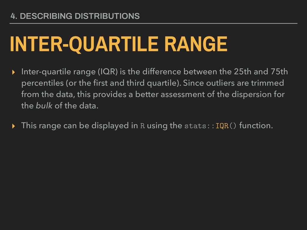
101. INTER-QUARTILE RANGE ▸ Inter-quartile range (IQR) is the difference between the 25th and 75th percentiles (or the first and third quartile). Since outliers are trimmed from the data, this provides a better assessment of the dispersion for the bulk of the data. ▸ This range can be displayed in R using the stats::IQR() function. 4. DESCRIBING DISTRIBUTIONS
102. 4. DESCRIBING DISTRIBUTIONS RANGE & IQR x = [ 1, 3, 4, 16, 18, 19, 22, 36, 52, 64, 81 ] > range(x) [1] 1 81 > > max(x)-min(x) [1] 80 > > IQR(x) [1] 34
103. 4. DESCRIBING DISTRIBUTIONS WHAT TO USE WHEN (GENERALLY!) Type Mode Median Mean Range IQR Binary Yes - Yes - - Categorical Yes - - - - Ordinal* Yes Yes Yes Yes - Continuous Yes Yes Yes Yes Yes * remember that the values assigned to ordinal variables will always affect statistics
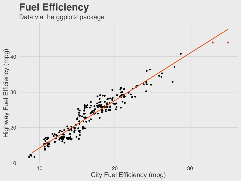
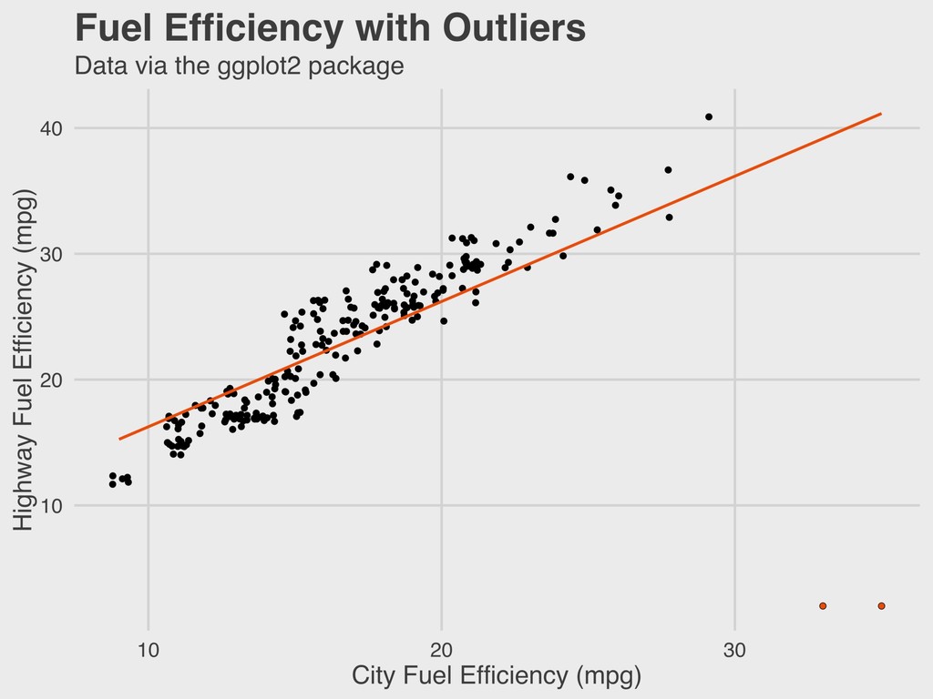
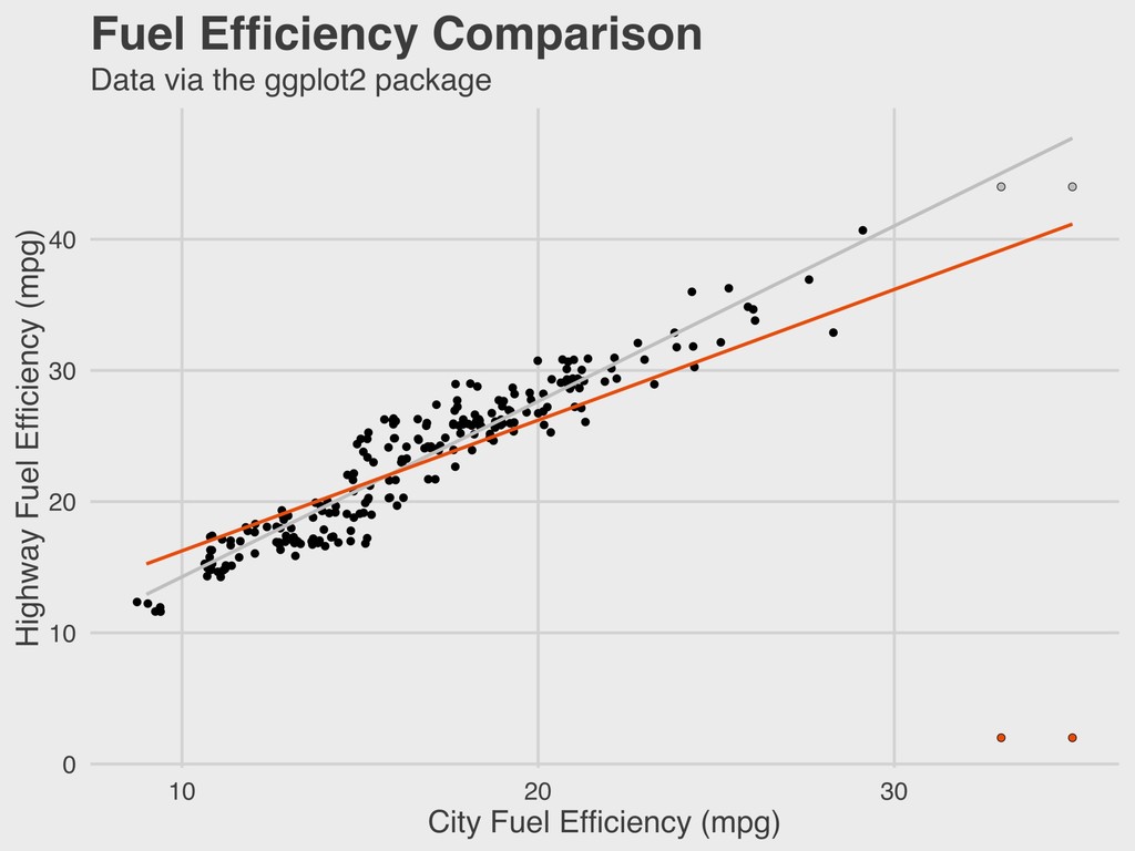
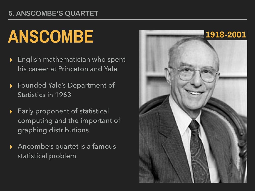
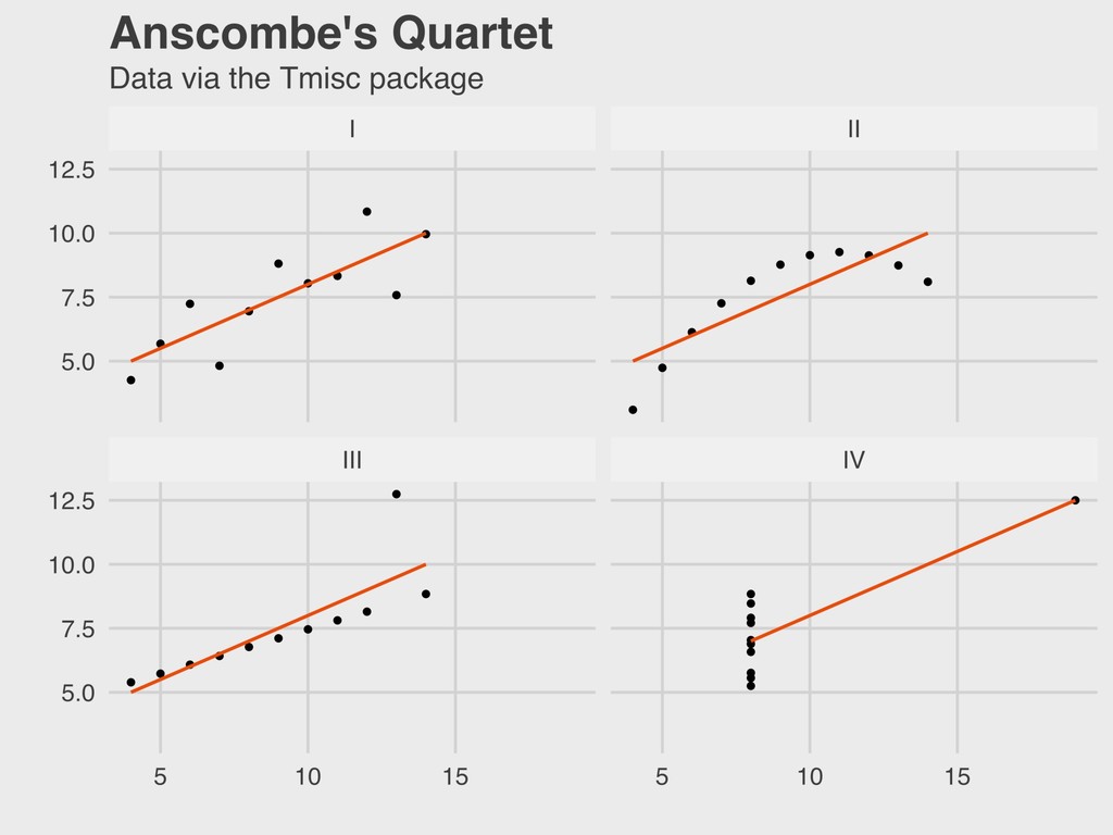
104. ▸ English mathematician who spent his career at Princeton and Yale ▸ Founded Yale’s Department of Statistics in 1963 ▸ Early proponent of statistical computing and the important of graphing distributions ▸ Ancombe’s quartet is a famous statistical problem 5. ANSCOMBE’S QUARTET ANSCOMBE 1918-2001
105. 5. ANSCOMBE’S QUARTET ANSCOMBE’S QUARTET The quartet is made up for four pairs of x and y variables, each with nearly identical mean and standard deviations. mean(x1) = 9.000000
 sd(x1) = 3.316625 mean(y1) = 7.500909
 sd(y1) = 2.031568 mean(x2) = 9.000000
 sd(x2) = 3.316625 mean(y2) = 7.500909
 sd(y2) = 2.031657 mean(x3) = 9.000000
 sd(x3) = 3.316625 mean(y3) = 7.500000
 sd(y3) = 2.030424 mean(x4) = 9.000000
 sd(x4) = 3.316625 mean(y4) = 7.500909
 sd(y4) = 2.030579 PAIR 1 PAIR 3 PAIR 4 PAIR 2
107. DESCRIPTIVE STATS AND GETTING HELP IN R 5
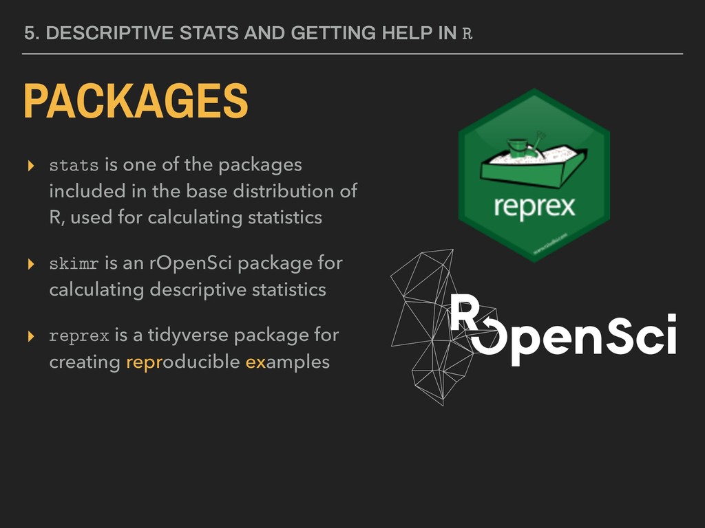
108. ▸ stats is one of the packages included in the base distribution of R, used for calculating statistics ▸ skimr is an rOpenSci package for calculating descriptive statistics ▸ reprex is a tidyverse package for creating reproducible examples 5. DESCRIPTIVE STATS AND GETTING HELP IN R PACKAGES
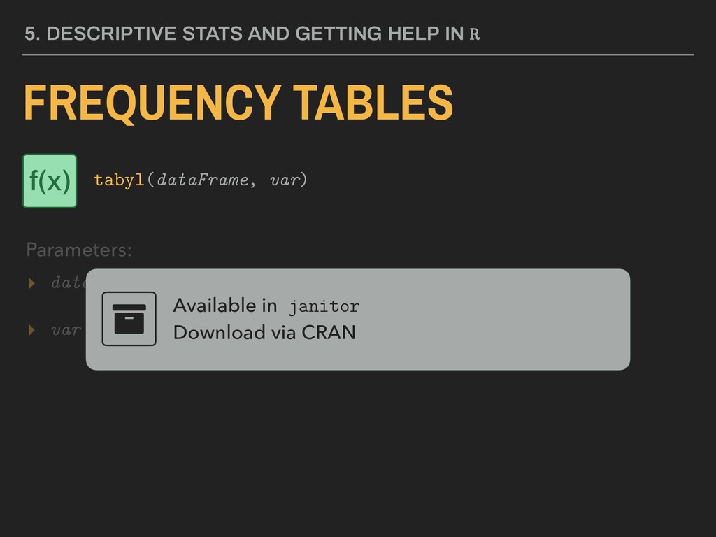
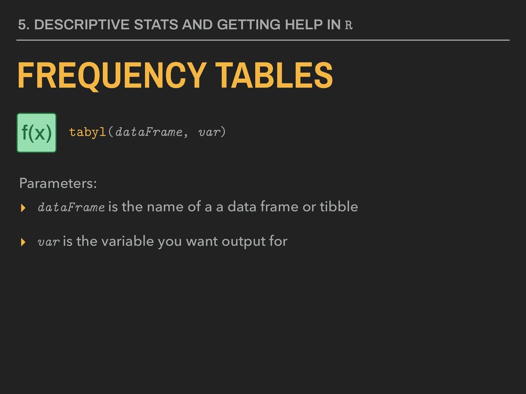
109. ▸ dataFrame is the name of a a data frame or tibble ▸ var is the variable you want output for Available in janitor
 Download via CRAN 5. DESCRIPTIVE STATS AND GETTING HELP IN R FREQUENCY TABLES Parameters: tabyl(dataFrame, var) f(x)
110. ▸ dataFrame is the name of a a data frame or tibble ▸ var is the variable you want output for 5. DESCRIPTIVE STATS AND GETTING HELP IN R FREQUENCY TABLES Parameters: tabyl(dataFrame, var) f(x)
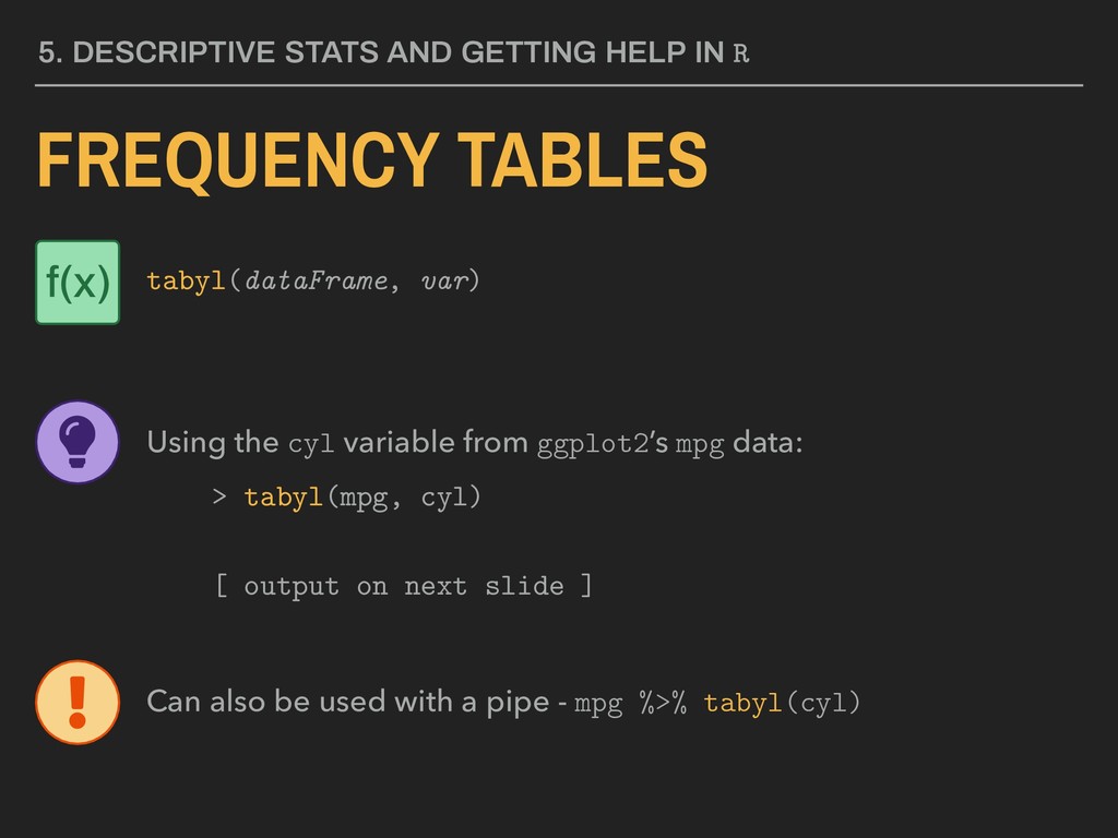
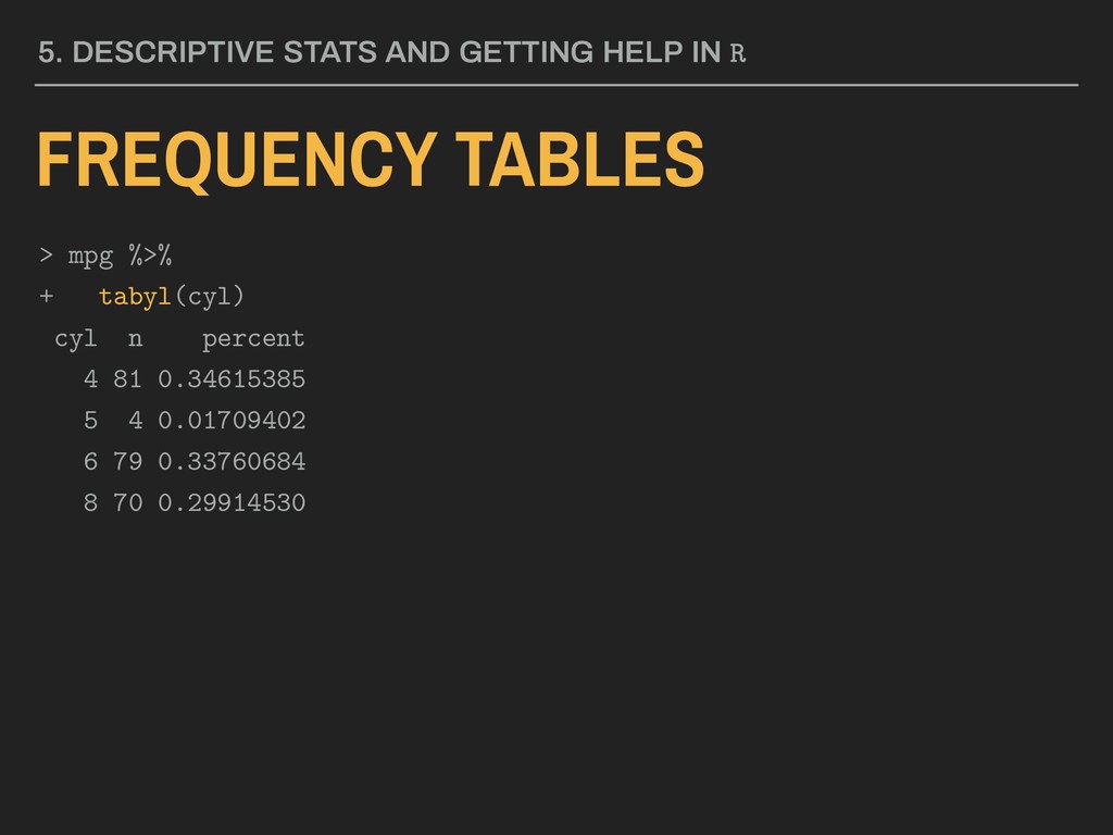
111. FREQUENCY TABLES 5. DESCRIPTIVE STATS AND GETTING HELP IN R tabyl(dataFrame, var) Using the cyl variable from ggplot2’s mpg data: > tabyl(mpg, cyl) [ output on next slide ] Can also be used with a pipe - mpg %>% tabyl(cyl) f(x)
112. FREQUENCY TABLES > mpg %>% + tabyl(cyl) cyl n percent 4 81 0.34615385 5 4 0.01709402 6 79 0.33760684 8 70 0.29914530 5. DESCRIPTIVE STATS AND GETTING HELP IN R
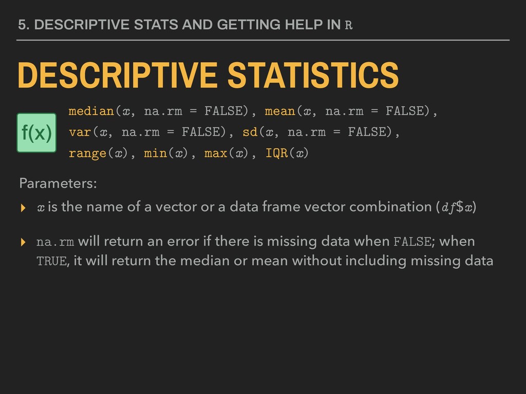
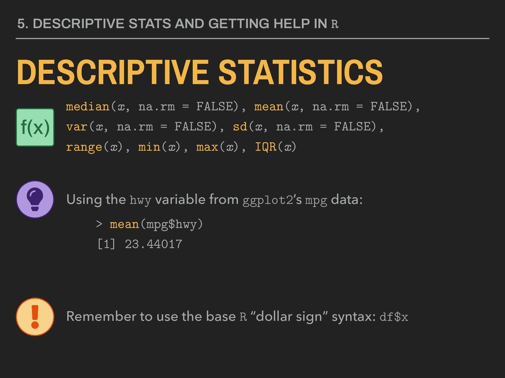
113. ▸ x is the name of a vector or a data frame vector combination (df$x) ▸ na.rm will return an error if there is missing data when FALSE; when TRUE, it will return the median or mean without including missing data Available in base and stats
 Download via CRAN 5. DESCRIPTIVE STATS AND GETTING HELP IN R DESCRIPTIVE STATISTICS Parameters: median(x, na.rm = FALSE), mean(x, na.rm = FALSE), var(x, na.rm = FALSE), sd(x, na.rm = FALSE), range(x), min(x), max(x), IQR(x) f(x)
114. ▸ x is the name of a vector or a data frame vector combination (df$x) ▸ na.rm will return an error if there is missing data when FALSE; when TRUE, it will return the median or mean without including missing data 5. DESCRIPTIVE STATS AND GETTING HELP IN R DESCRIPTIVE STATISTICS Parameters: median(x, na.rm = FALSE), mean(x, na.rm = FALSE), var(x, na.rm = FALSE), sd(x, na.rm = FALSE), range(x), min(x), max(x), IQR(x) f(x)
115. DESCRIPTIVE STATISTICS 5. DESCRIPTIVE STATS AND GETTING HELP IN R median(x, na.rm = FALSE), mean(x, na.rm = FALSE), var(x, na.rm = FALSE), sd(x, na.rm = FALSE), range(x), min(x), max(x), IQR(x) Using the hwy variable from ggplot2’s mpg data: > mean(mpg$hwy) [1] 23.44017 Remember to use the base R “dollar sign” syntax: df$x f(x)
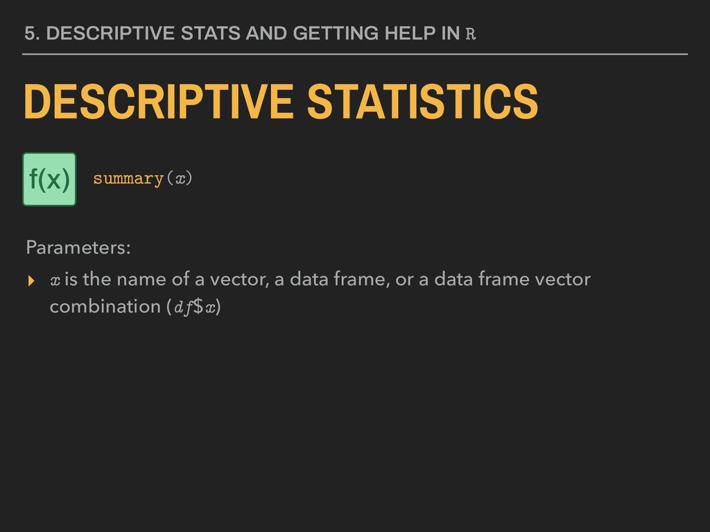
116. ▸ x is the name of a vector or a data frame vector combination (df$x) Available in stats
 Download via CRAN 5. DESCRIPTIVE STATS AND GETTING HELP IN R DESCRIPTIVE STATISTICS Parameters: summary(x) f(x)
117. ▸ x is the name of a vector, a data frame, or a data frame vector combination (df$x) 5. DESCRIPTIVE STATS AND GETTING HELP IN R DESCRIPTIVE STATISTICS Parameters: summary(x) f(x)
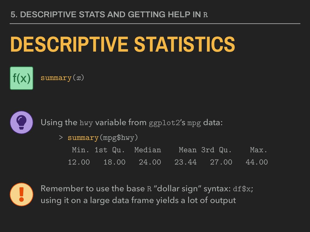
118. DESCRIPTIVE STATISTICS 5. DESCRIPTIVE STATS AND GETTING HELP IN R summary(x) Using the hwy variable from ggplot2’s mpg data: > summary(mpg$hwy) Min. 1st Qu. Median Mean 3rd Qu. Max. 12.00 18.00 24.00 23.44 27.00 44.00 Remember to use the base R “dollar sign” syntax: df$x;
 using it on a large data frame yields a lot of output f(x)
119. ▸ “rOpenSci fosters a culture that values open and reproducible research using shared data and reusable software” (rOpenSci 2018) ▸ rOpenSci: • Reviews and helps support packages to accessing scientific data • Hosts “unconferences” 5. DESCRIPTIVE STATS AND GETTING HELP IN R ROPENSCI
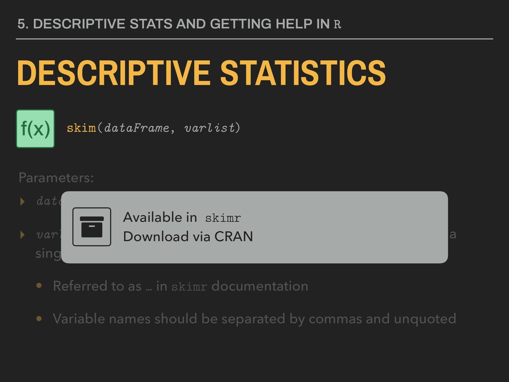
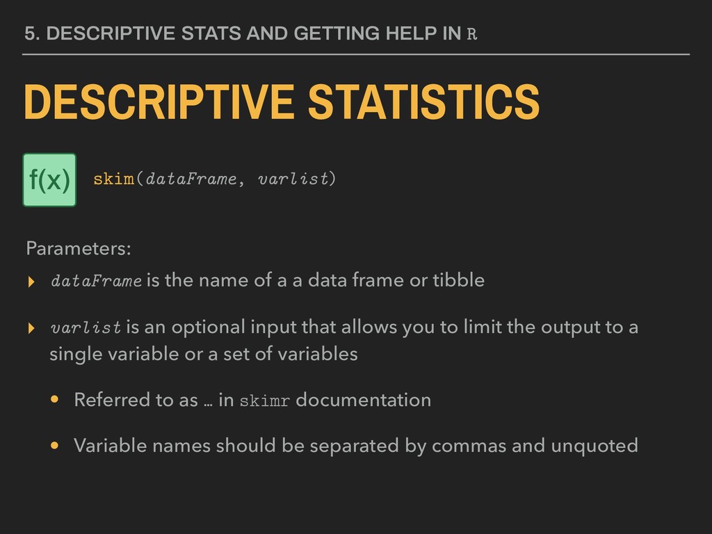
120. ▸ dataFrame is the name of a a data frame or tibble ▸ varlist is an optional input that allows you to limit the output to a single variable or a set of variables • Referred to as … in skimr documentation • Variable names should be separated by commas and unquoted Available in skimr
 Download via CRAN 5. DESCRIPTIVE STATS AND GETTING HELP IN R DESCRIPTIVE STATISTICS Parameters: skim(dataFrame, varlist) f(x)
121. ▸ dataFrame is the name of a a data frame or tibble ▸ varlist is an optional input that allows you to limit the output to a single variable or a set of variables • Referred to as … in skimr documentation • Variable names should be separated by commas and unquoted 5. DESCRIPTIVE STATS AND GETTING HELP IN R DESCRIPTIVE STATISTICS Parameters: skim(dataFrame, varlist) f(x)
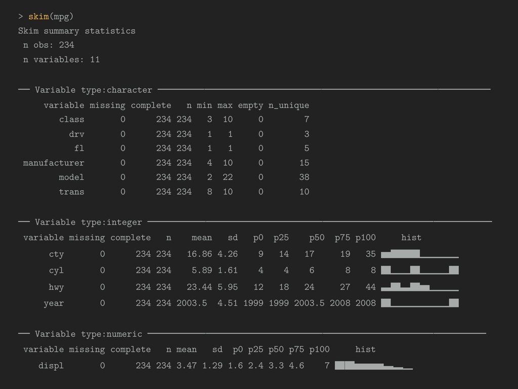
122. DESCRIPTIVE STATISTICS 5. DESCRIPTIVE STATS AND GETTING HELP IN R skim(dataFrame, varlist) Using ggplot2’s mpg data: > skim(mpg) [ output on next slide ] Output in notebooks will sometimes not fit on one row and will wrap when those notebooks are knit. f(x)
123. > skim(mpg) Skim summary statistics n obs: 234 n variables: 11 "" Variable type:character """"""""""""""""""""""""""""""""""""""""""""""""""""""""" variable missing complete n min max empty n_unique class 0 234 234 3 10 0 7 drv 0 234 234 1 1 0 3 fl 0 234 234 1 1 0 5 manufacturer 0 234 234 4 10 0 15 model 0 234 234 2 22 0 38 trans 0 234 234 8 10 0 10 "" Variable type:integer """"""""""""""""""""""""""""""""""""""""""""""""""""""""""" variable missing complete n mean sd p0 p25 p50 p75 p100 hist cty 0 234 234 16.86 4.26 9 14 17 19 35 ▅▇▇▇▁▁▁▁ cyl 0 234 234 5.89 1.61 4 4 6 8 8 ▇▁▁▇▁▁▁▇ hwy 0 234 234 23.44 5.95 12 18 24 27 44 ▃▇▃▇▅▁▁▁ year 0 234 234 2003.5 4.51 1999 1999 2003.5 2008 2008 ▇▁▁▁▁▁▁▇ "" Variable type:numeric """""""""""""""""""""""""""""""""""""""""""""""""""""""""" variable missing complete n mean sd p0 p25 p50 p75 p100 hist displ 0 234 234 3.47 1.29 1.6 2.4 3.3 4.6 7 ▇▇▅▅▅▃▂▁
124. Available in reprex
 Download via CRAN 5. DESCRIPTIVE STATS AND GETTING HELP IN R REPRODUCIBLE EXAMPLES reprex() f(x) See the workflow handout for implementation details!
125. 6 BACK 
 MATTER
126. AGENDA REVIEW 6. BACK MATTER 2. Getting Organized 3. Visualizing Distributions 4. Describing Distributions 5. Descriptive Stats and Getting Help in R
127. Final project progress report due at Lecture-05; focus on Vignettes 2 & 4 REMINDERS 6. BACK MATTER Lab-02, PS-01, and LP-04 are due before Lecture-04 Final project data for the 2016 General Social Survey is now available on GitHub (linked to via “Final Project” page on course website; for SOC 4015 only)