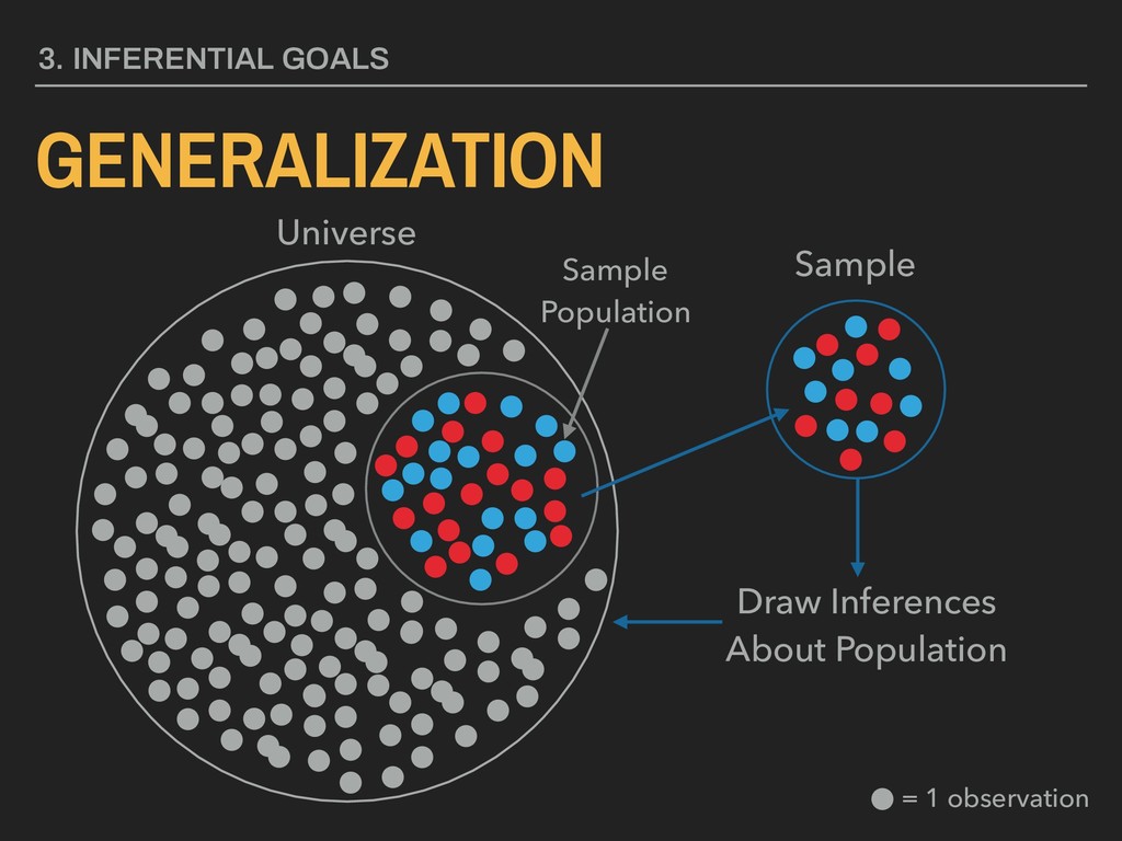
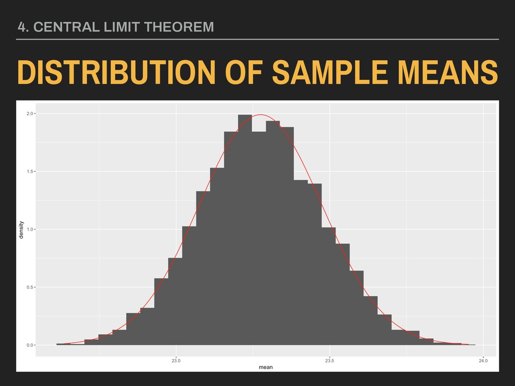
Lecture slides for Lecture 06 of the Saint Louis University Course Quantitative Analysis: Applied Inferential Statistics. These slides cover the central limit theorem, confidence intervals, and more details on hypothesis testing.
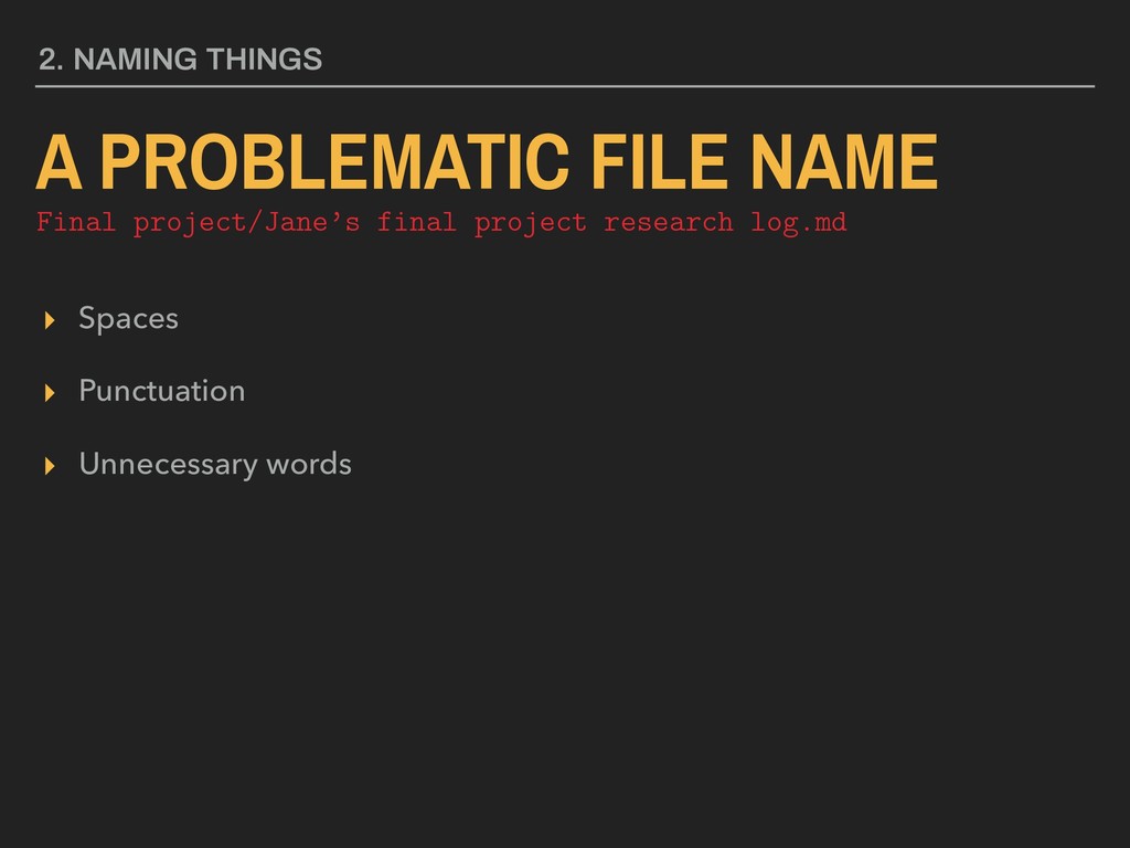
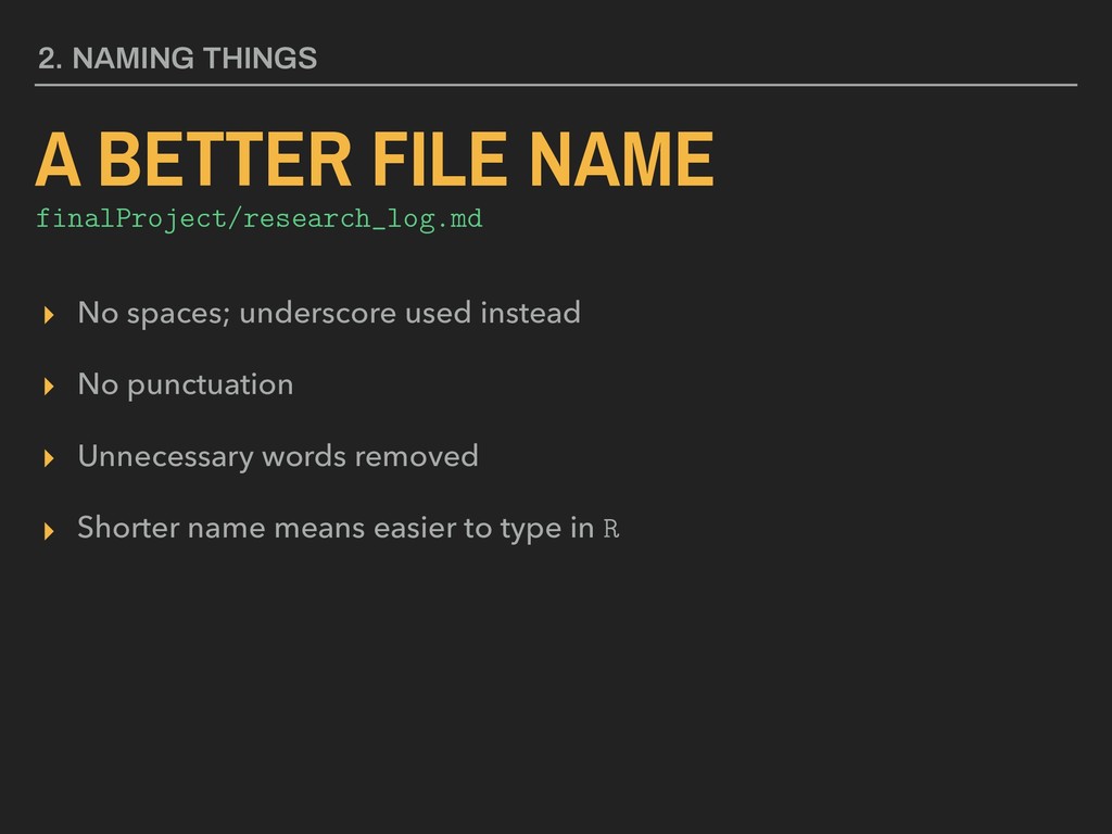
Naming simplified ▸ No spaces; camel case used instead ▸ Using 01 and 02 allows computer to present file names in proper order through Windows File Explorer or macOS Finder
Naming simplified ▸ No spaces; dashes and underscores used instead ▸ Using dates in year-month-day formatting allows computer to present file names in proper order through Windows File Explorer or macOS Finder
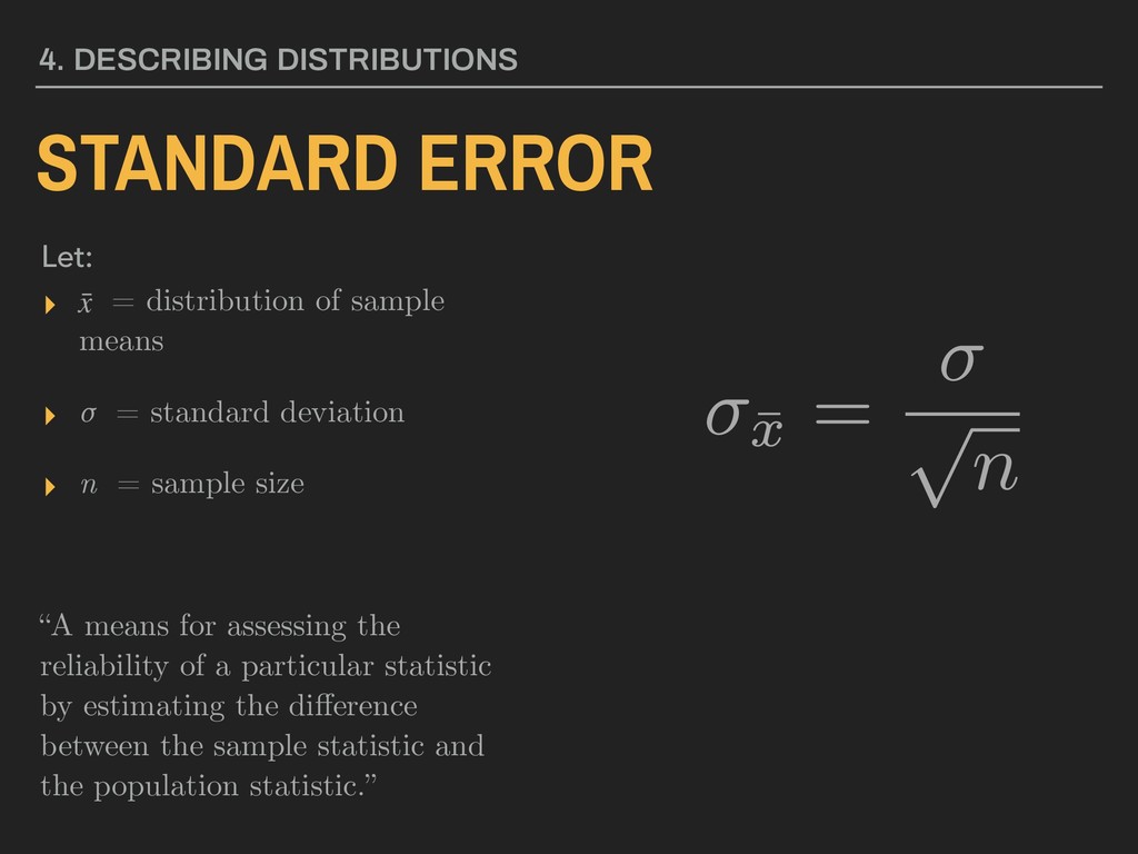
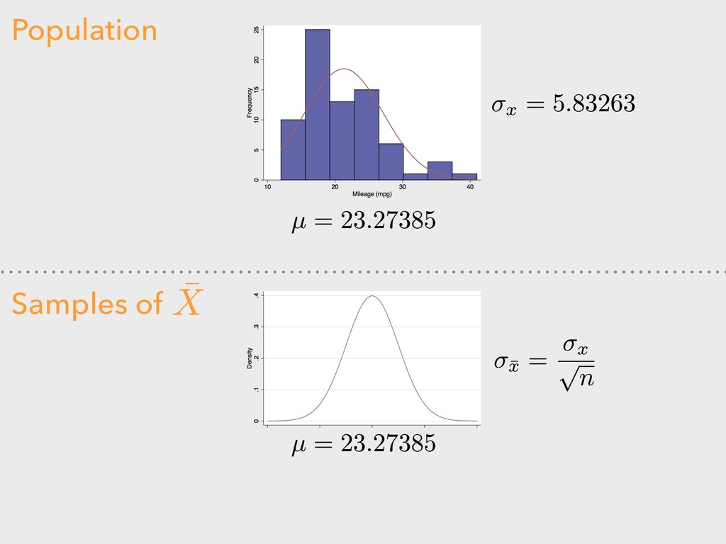
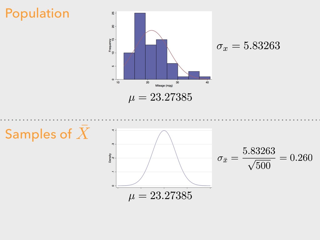
standard deviation ▸ n = sample size “A means for assessing the reliability of a particular statistic by estimating the difference between the sample statistic and the population statistic.” 4. DESCRIBING DISTRIBUTIONS Let: STANDARD ERROR ¯ x
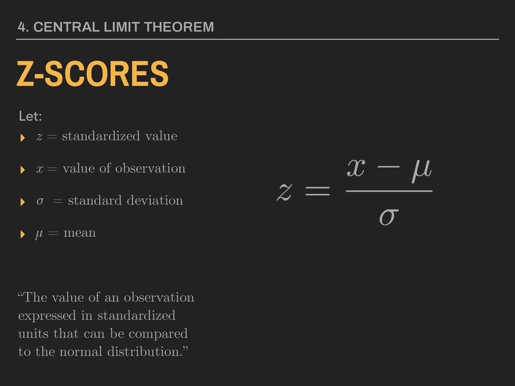
observation ▸ σ = standard deviation ▸ µ = mean “The value of an observation expressed in standardized units that can be compared to the normal distribution.” 4. CENTRAL LIMIT THEOREM Let: Z-SCORES
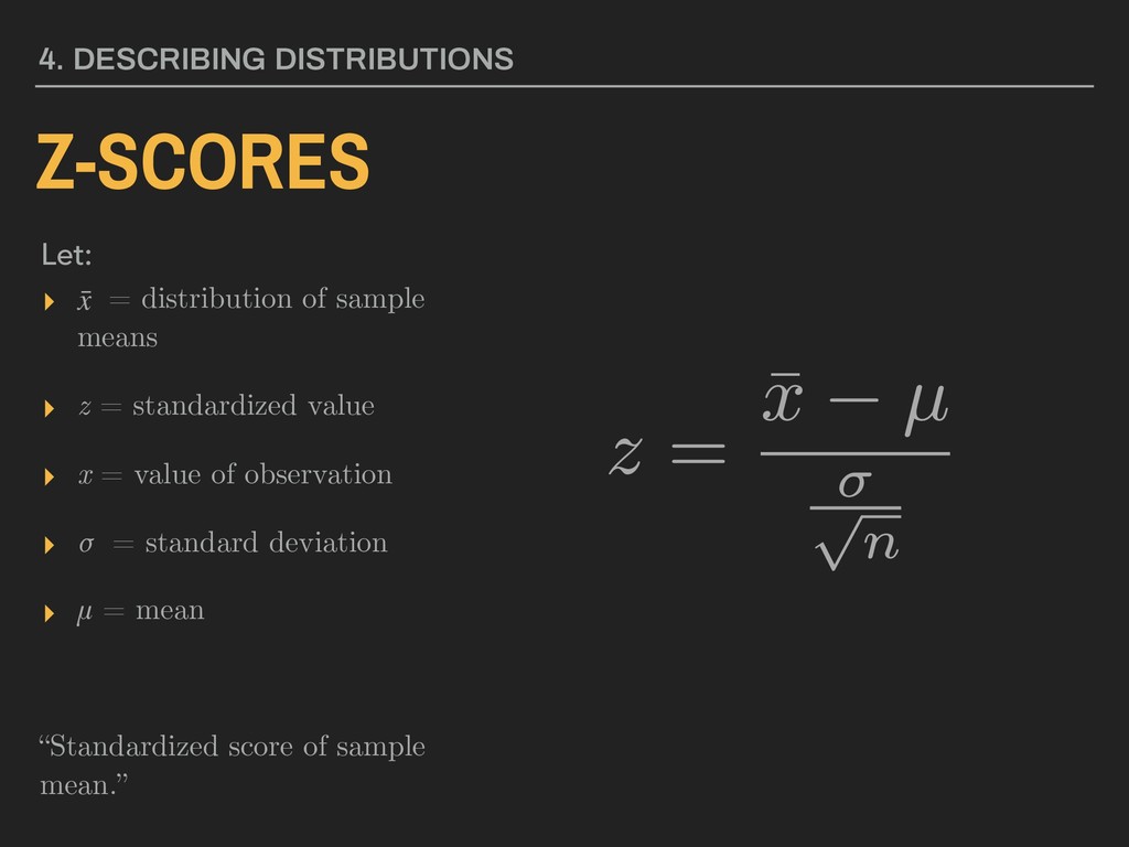
standardized value ▸ x = value of observation ▸ σ = standard deviation ▸ µ = mean “Standardized score of sample mean.” 4. DESCRIBING DISTRIBUTIONS Let: Z-SCORES ¯ x
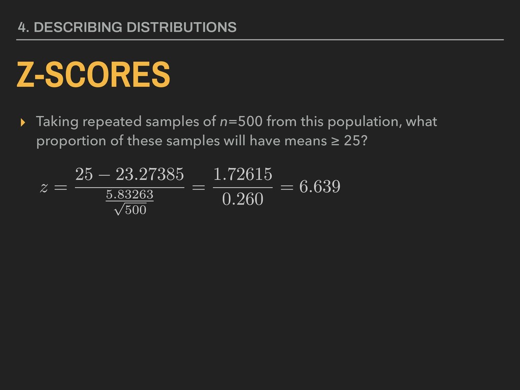
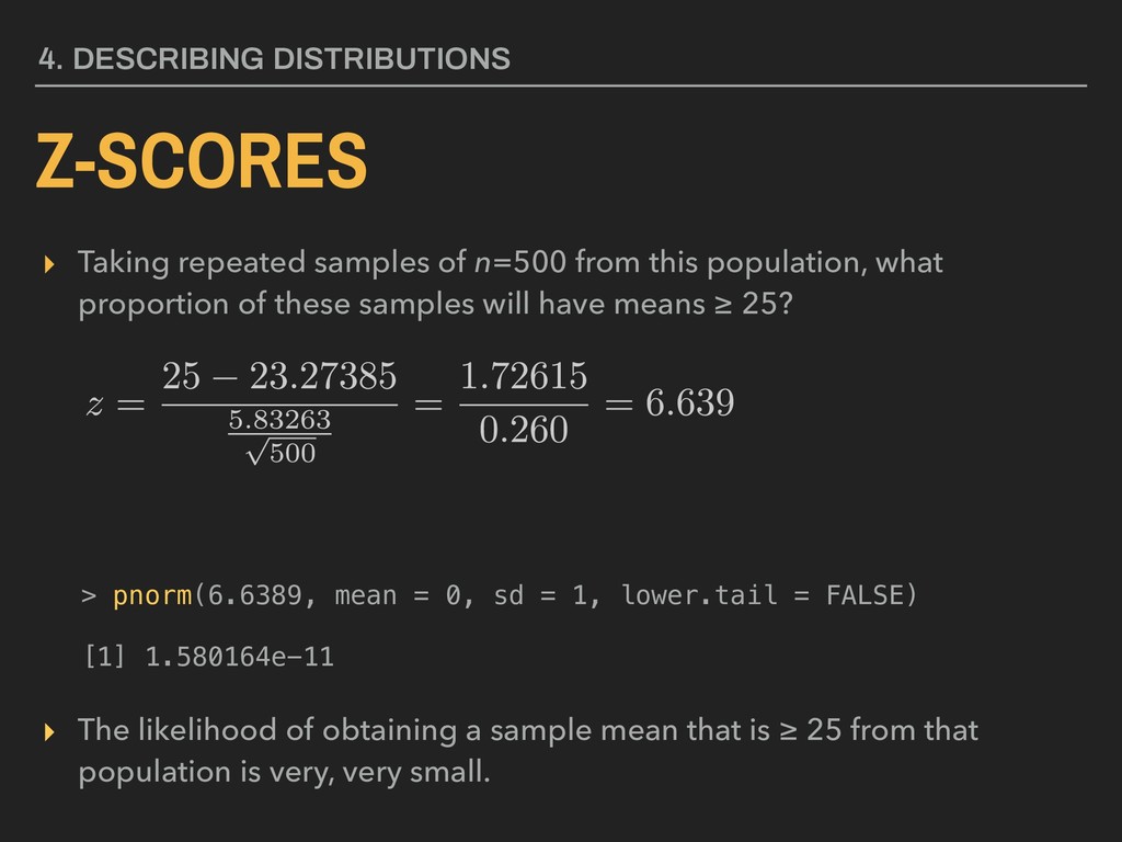
what proportion of these samples will have means ≥ 25? 4. DESCRIBING DISTRIBUTIONS > pnorm(6.6389, mean = 0, sd = 1, lower.tail = FALSE) [1] 1.580164e-11 ▸ The likelihood of obtaining a sample mean that is ≥ 25 from that population is very, very small.
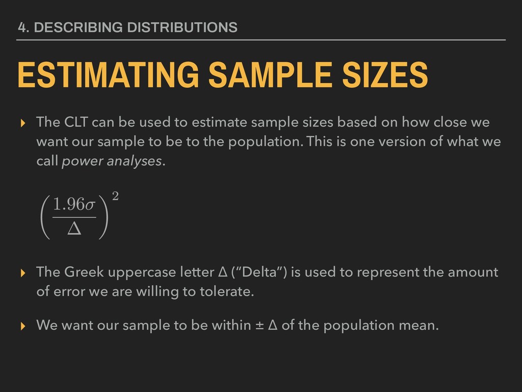
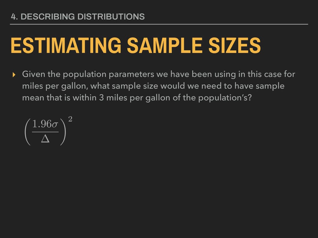
estimate sample sizes based on how close we want our sample to be to the population. This is one version of what we call power analyses. ▸ The Greek uppercase letter ∆ (“Delta”) is used to represent the amount of error we are willing to tolerate. ▸ We want our sample to be within ± ∆ of the population mean. 4. DESCRIBING DISTRIBUTIONS
been using in this case for miles per gallon, what sample size would we need to have sample mean that is within 3 miles per gallon of the population’s? 4. DESCRIBING DISTRIBUTIONS
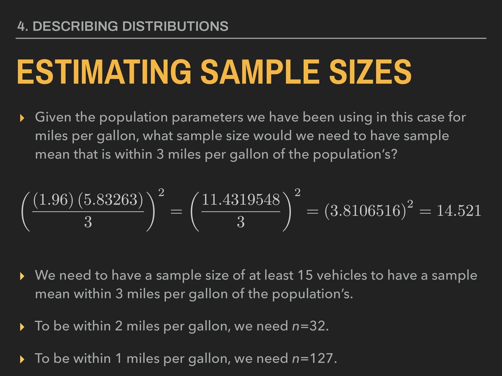
been using in this case for miles per gallon, what sample size would we need to have sample mean that is within 3 miles per gallon of the population’s? 4. DESCRIBING DISTRIBUTIONS ▸ We need to have a sample size of at least 15 vehicles to have a sample mean within 3 miles per gallon of the population’s. ▸ To be within 2 miles per gallon, we need n=32. ▸ To be within 1 miles per gallon, we need n=127.
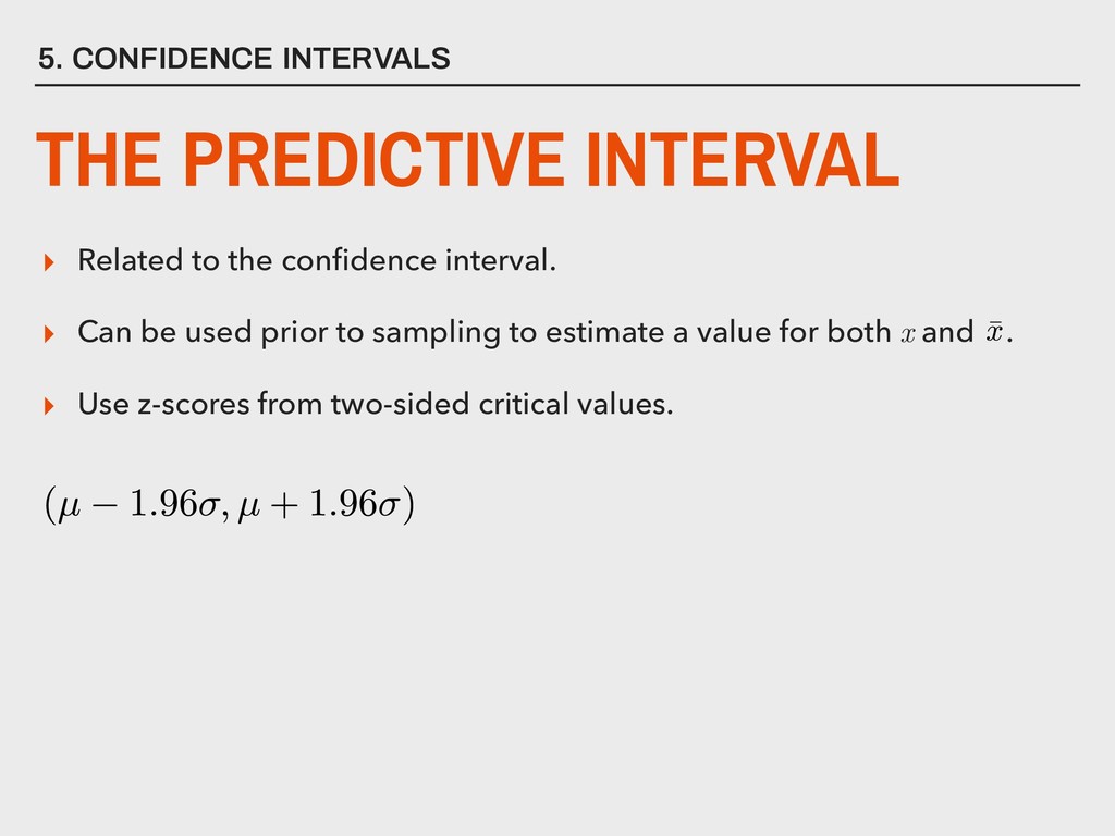
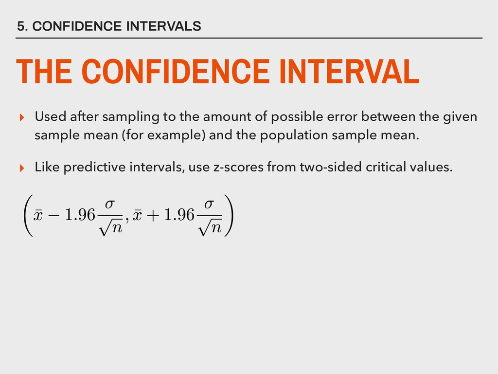
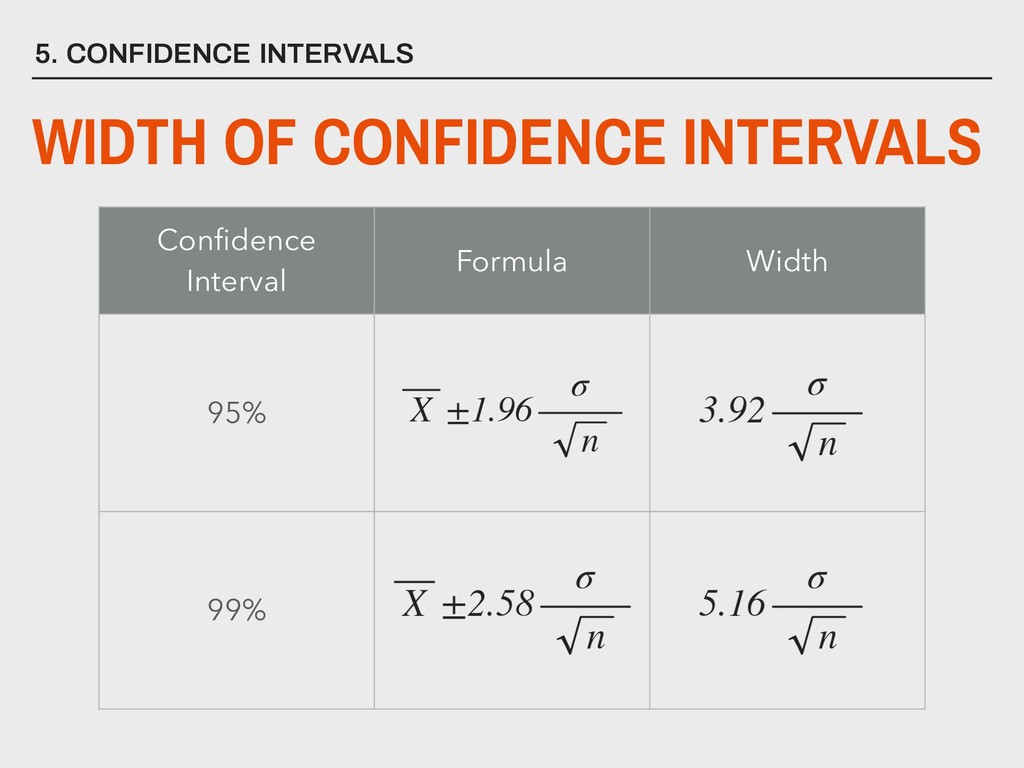
to the amount of possible error between the given sample mean (for example) and the population sample mean. ▸ Like predictive intervals, use z-scores from two-sided critical values.
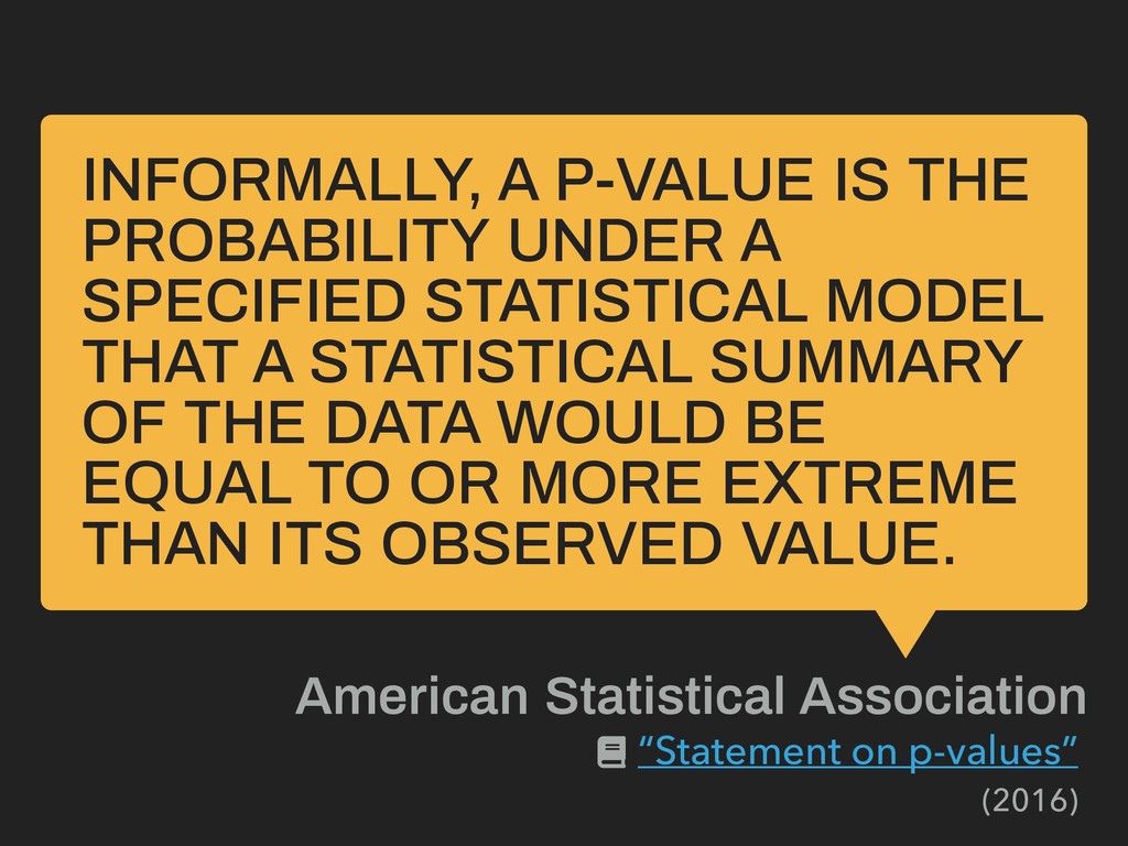
MODEL THAT A STATISTICAL SUMMARY OF THE DATA WOULD BE EQUAL TO OR MORE EXTREME THAN ITS OBSERVED VALUE. American Statistical Association “Statement on p-values” (2016)
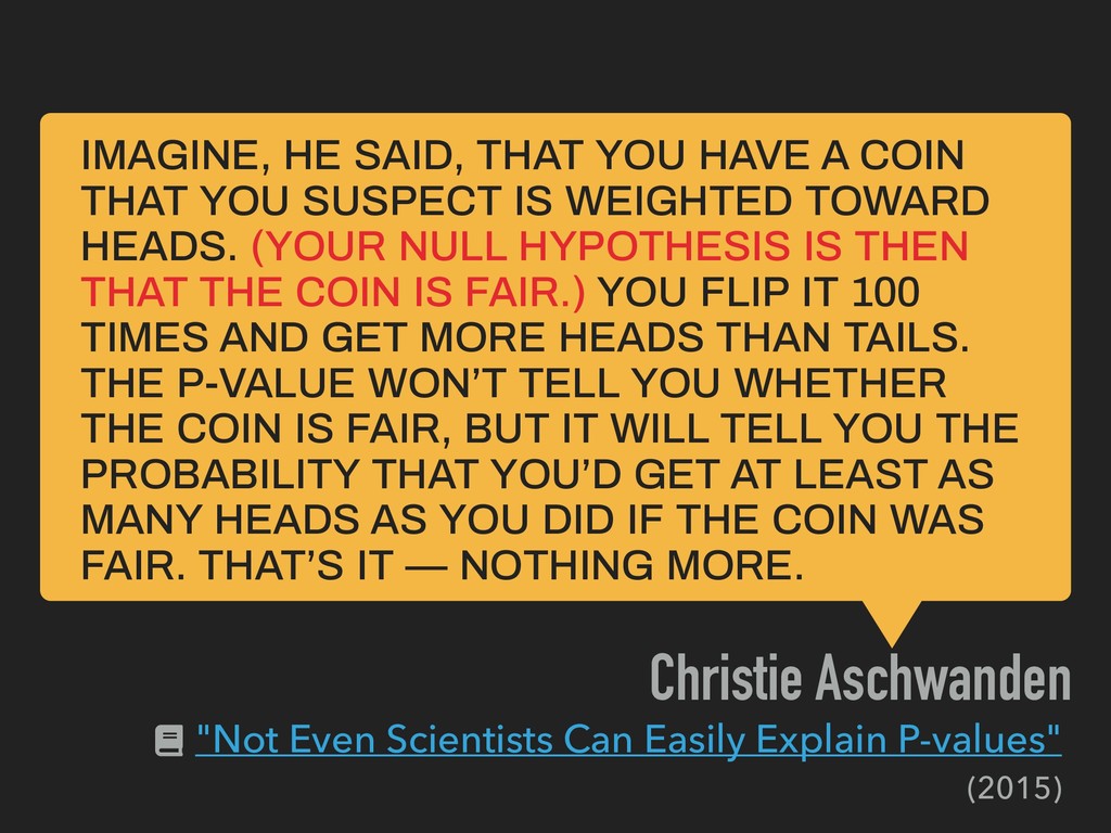
SUSPECT IS WEIGHTED TOWARD HEADS. (YOUR NULL HYPOTHESIS IS THEN THAT THE COIN IS FAIR.) YOU FLIP IT 100 TIMES AND GET MORE HEADS THAN TAILS. THE P-VALUE WON’T TELL YOU WHETHER THE COIN IS FAIR, BUT IT WILL TELL YOU THE PROBABILITY THAT YOU’D GET AT LEAST AS MANY HEADS AS YOU DID IF THE COIN WAS FAIR. THAT’S IT — NOTHING MORE. Christie Aschwanden "Not Even Scientists Can Easily Explain P-values" (2015)
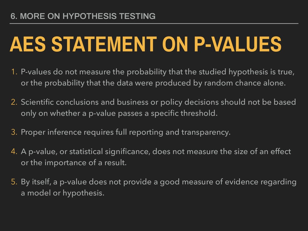
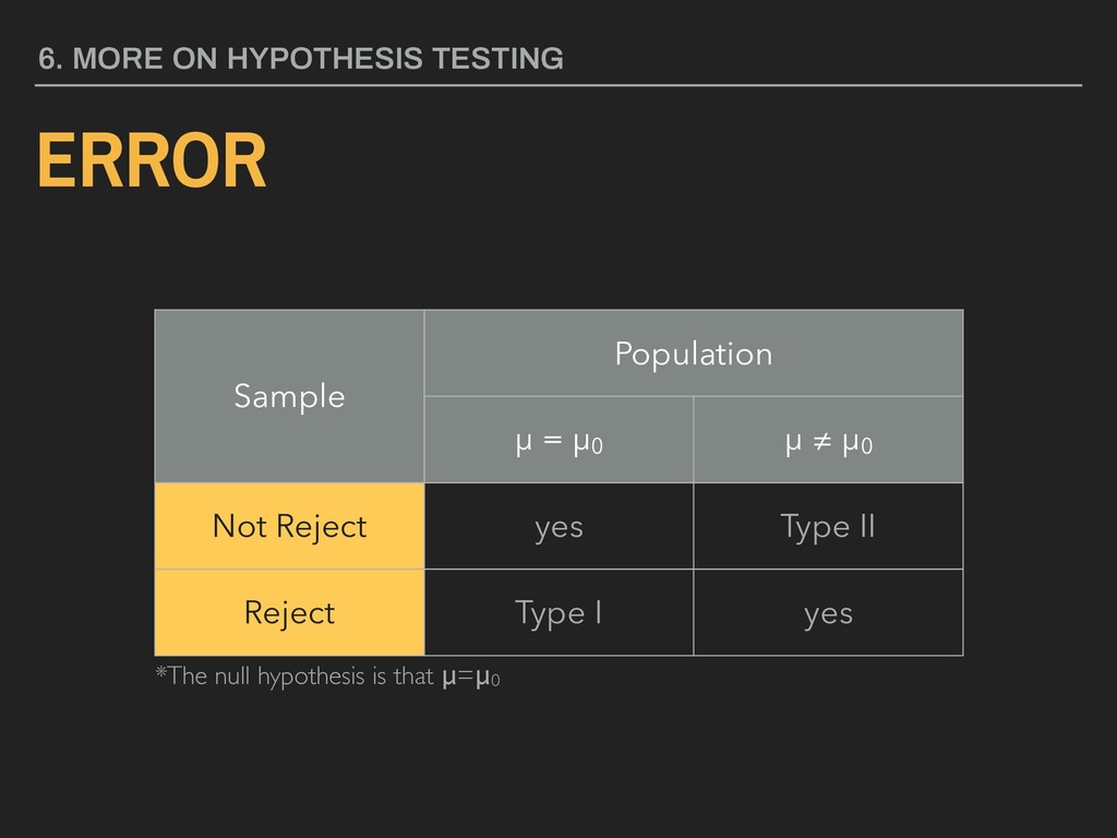
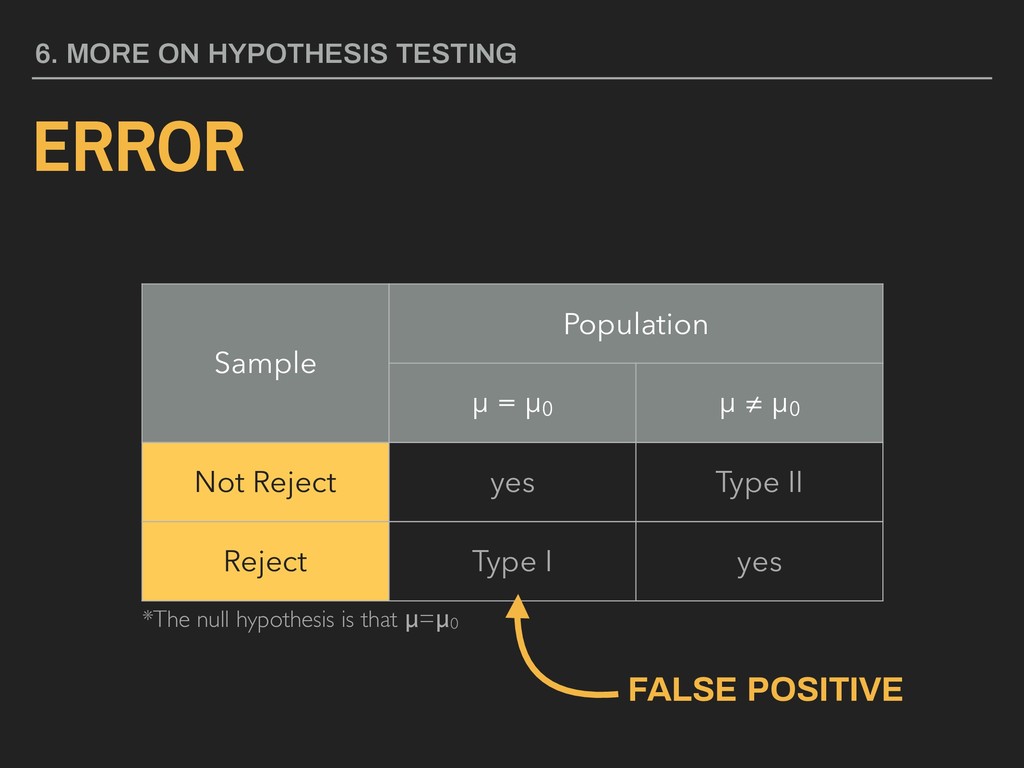
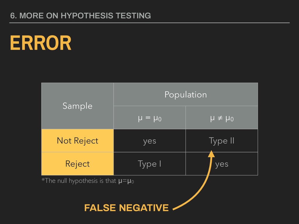
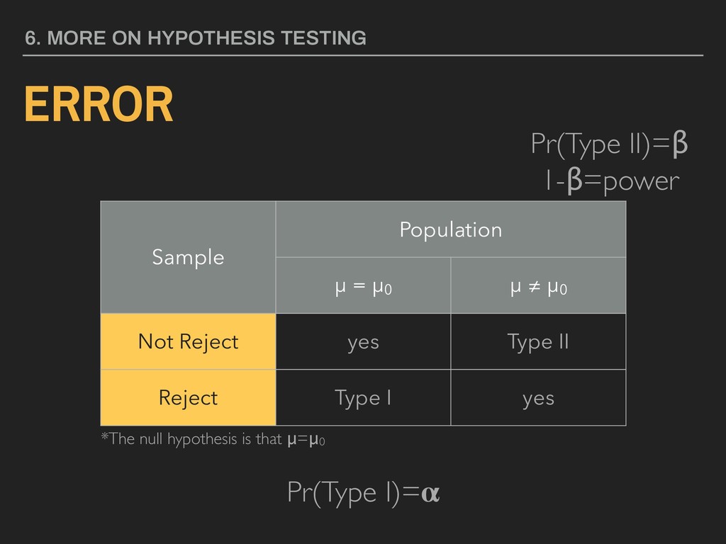
probability that the studied hypothesis is true, or the probability that the data were produced by random chance alone. 2. Scientific conclusions and business or policy decisions should not be based only on whether a p-value passes a specific threshold. 3. Proper inference requires full reporting and transparency. 4. A p-value, or statistical significance, does not measure the size of an effect or the importance of a result. 5. By itself, a p-value does not provide a good measure of evidence regarding a model or hypothesis. 6. MORE ON HYPOTHESIS TESTING
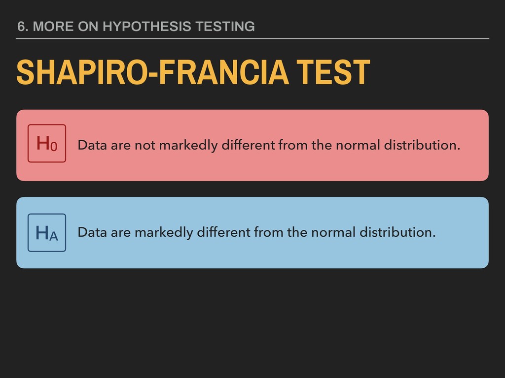
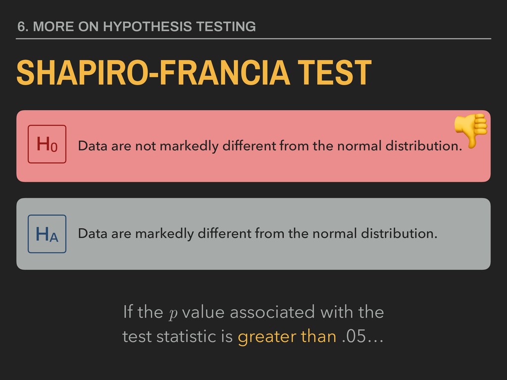
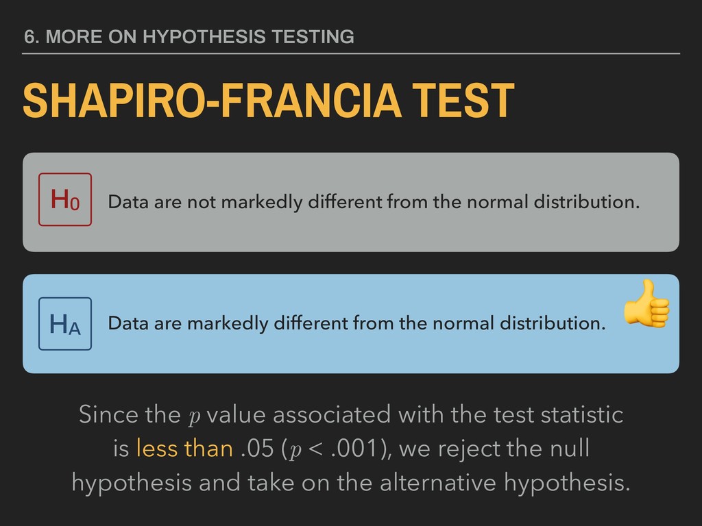
markedly different from the normal distribution. H0 Data are markedly different from the normal distribution. HA If the p value associated with the test statistic is greater than .05…
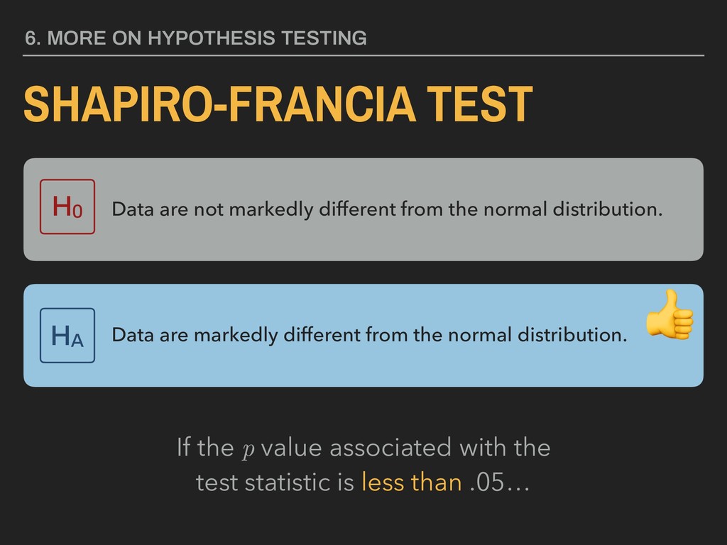
markedly different from the normal distribution. H0 Data are markedly different from the normal distribution. HA If the p value associated with the test statistic is less than .05…
markedly different from the normal distribution. H0 Data are markedly different from the normal distribution. HA Since the p value associated with the test statistic is less than .05 (p < .001), we reject the null hypothesis and take on the alternative hypothesis.
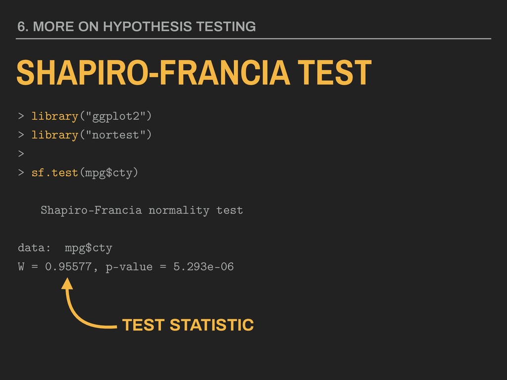
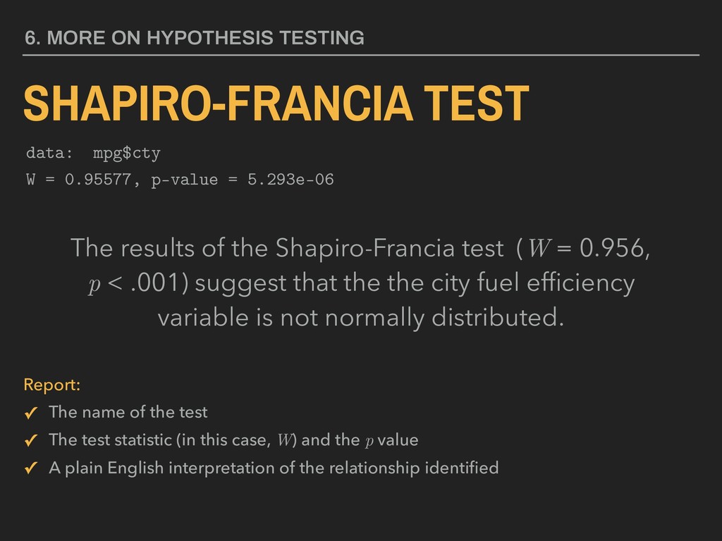
the Shapiro-Francia test (W = 0.956, p < .001) suggest that the the city fuel efficiency variable is not normally distributed. data: mpg$cty W = 0.95577, p-value = 5.293e-06 Report: ✓ The name of the test ✓ The test statistic (in this case, W) and the p value ✓ A plain English interpretation of the relationship identified
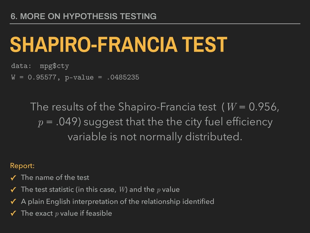
the Shapiro-Francia test (W = 0.956, p = .049) suggest that the the city fuel efficiency variable is not normally distributed. data: mpg$cty W = 0.95577, p-value = .0485235 Report: ✓ The name of the test ✓ The test statistic (in this case, W) and the p value ✓ A plain English interpretation of the relationship identified ✓ The exact p value if feasible
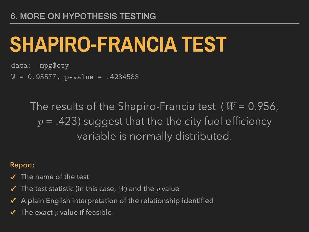
the Shapiro-Francia test (W = 0.956, p = .423) suggest that the the city fuel efficiency variable is normally distributed. data: mpg$cty W = 0.95577, p-value = .4234583 Report: ✓ The name of the test ✓ The test statistic (in this case, W) and the p value ✓ A plain English interpretation of the relationship identified ✓ The exact p value if feasible
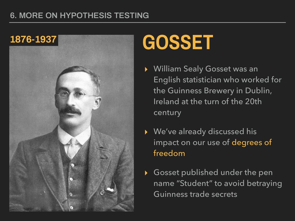
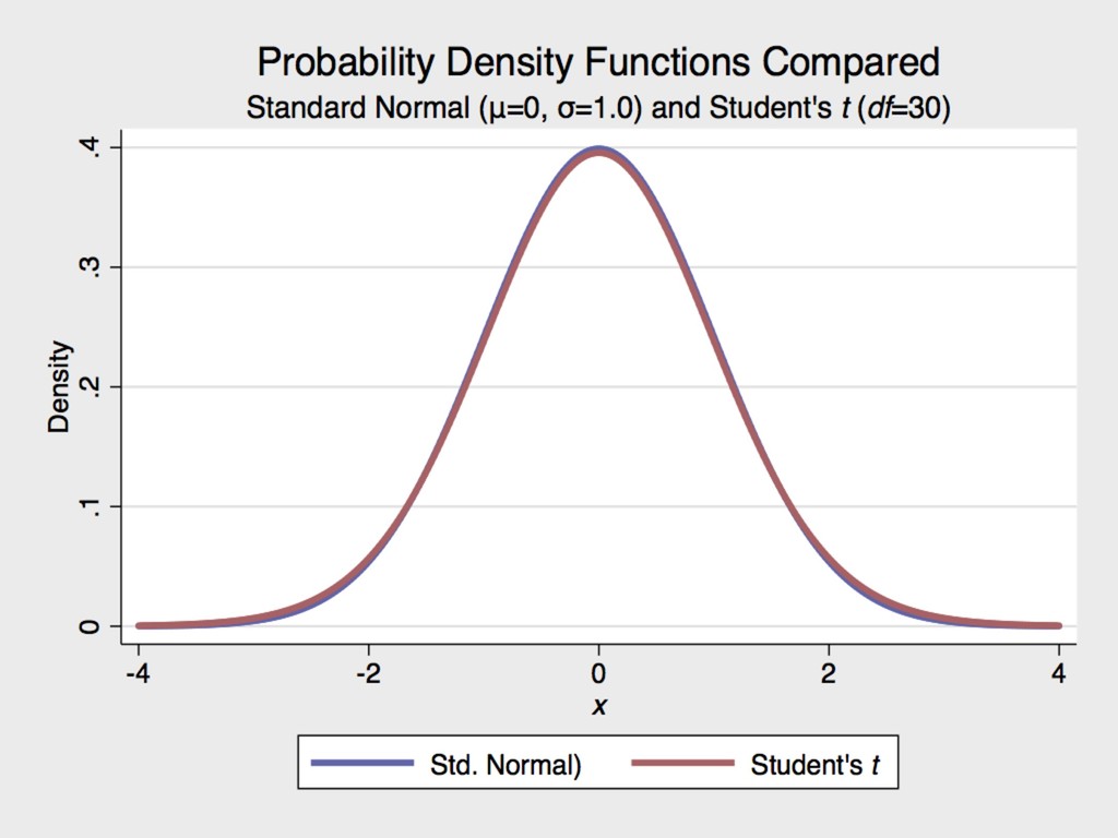
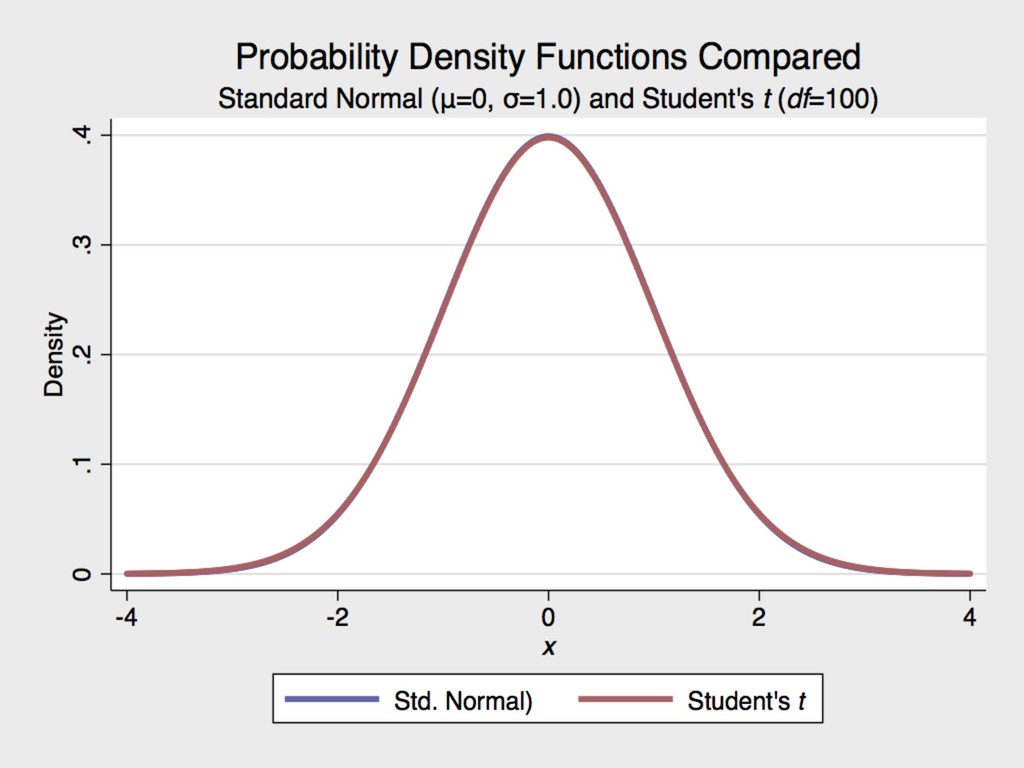
for the Guinness Brewery in Dublin, Ireland at the turn of the 20th century ▸ We’ve already discussed his impact on our use of degrees of freedom ▸ Gosset published under the pen name “Student” to avoid betraying Guinness trade secrets 6. MORE ON HYPOTHESIS TESTING GOSSET 1876-1937
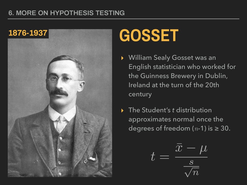
for the Guinness Brewery in Dublin, Ireland at the turn of the 20th century ▸ The Student’s t distribution approximates normal once the degrees of freedom (n-1) is ≥ 30. 6. MORE ON HYPOTHESIS TESTING GOSSET 1876-1937
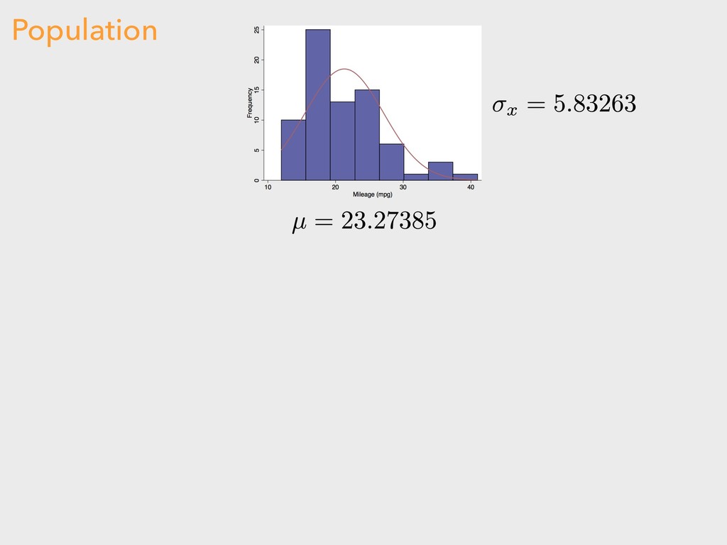
![COMPARING POPULATION TO SAMPLES > mean(autoData$combFE) [1] 23.27385 > sd(autoData$combFE)](https://files.speakerdeck.com/presentations/fee57d160dff4883b35ddefc565510b3/slide_25.jpg)