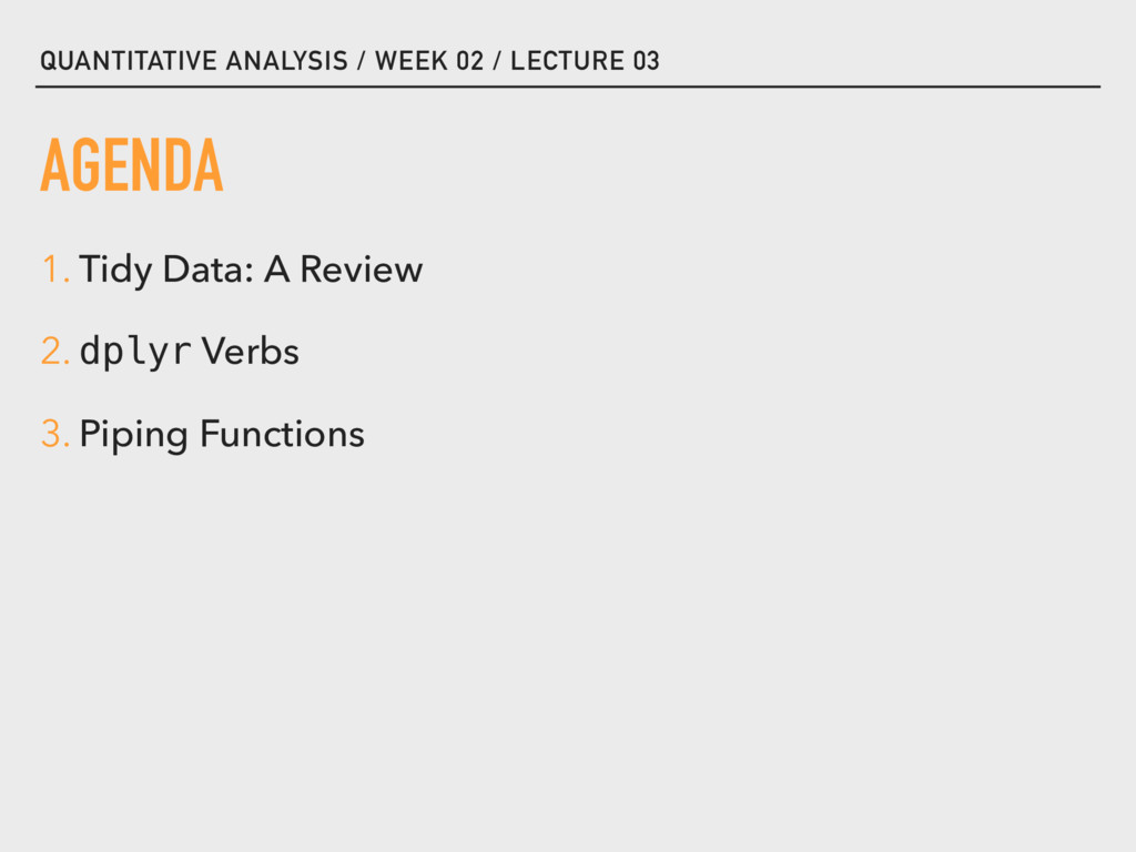
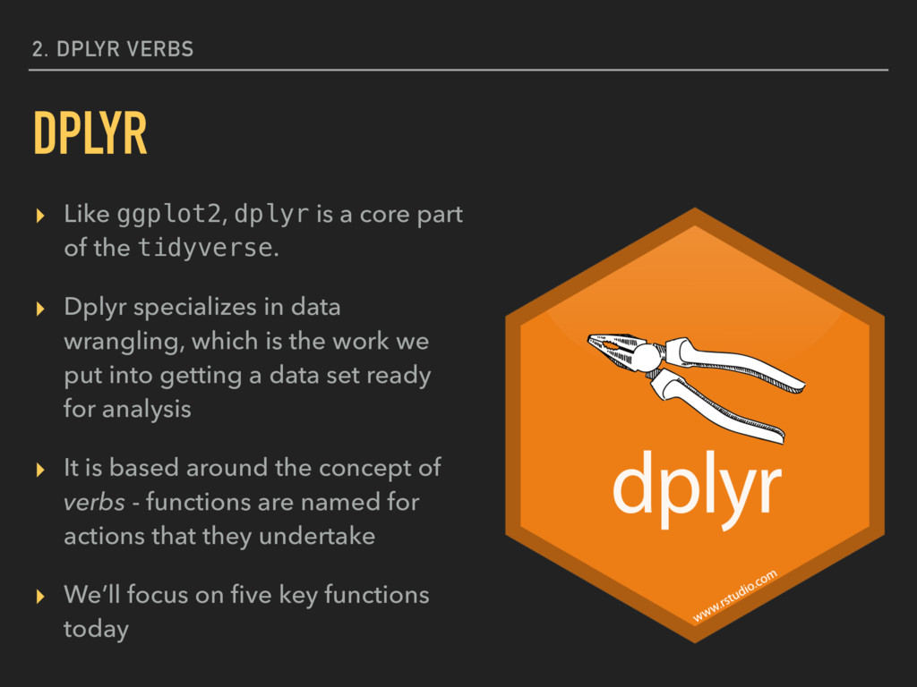
Lecture slides for Week 02, Lecture 03 of the Saint Louis University Course Quantitative Analysis: Applied Inferential Statistics. These slides cover the basics of the R package dplyr.
part of the tidyverse. ▸ Dplyr specializes in data wrangling, which is the work we put into getting a data set ready for analysis ▸ It is based around the concept of verbs - functions are named for actions that they undertake ▸ We’ll focus on five key functions today DPLYR
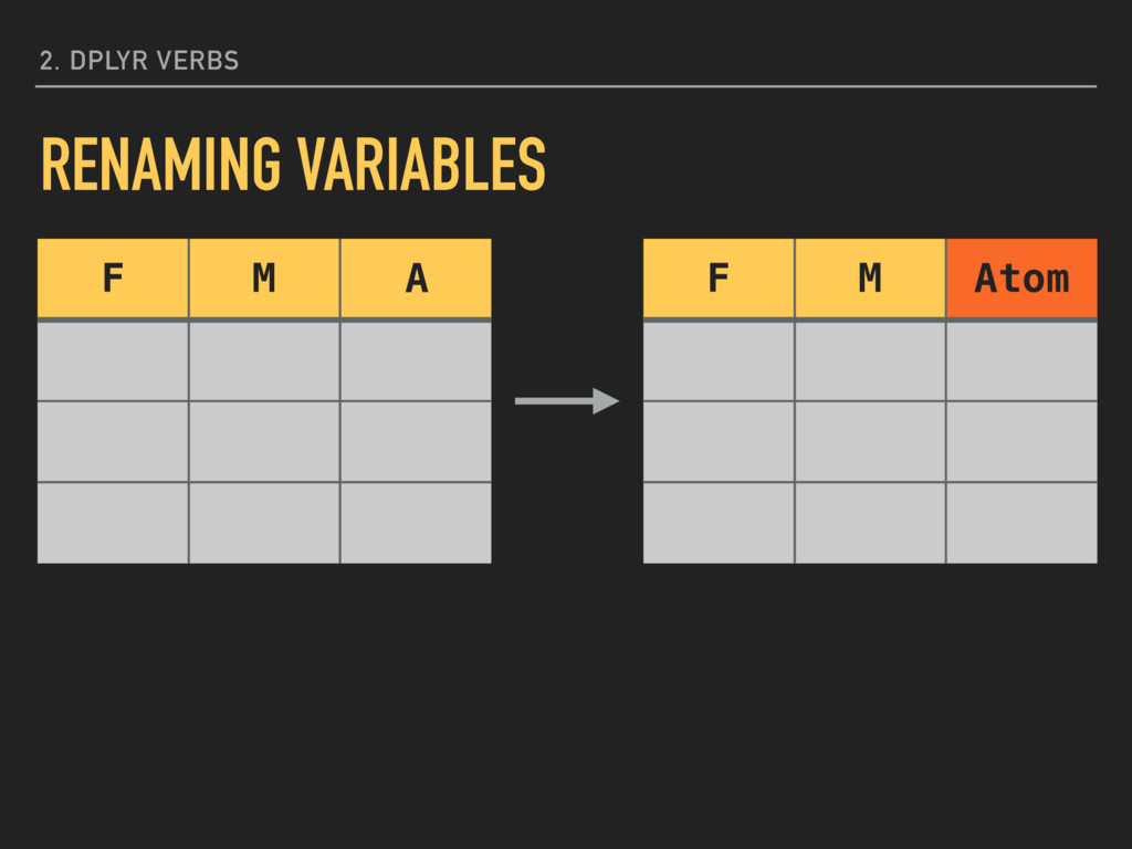
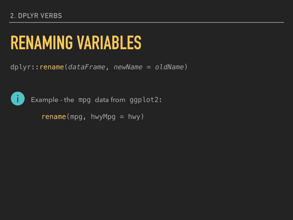
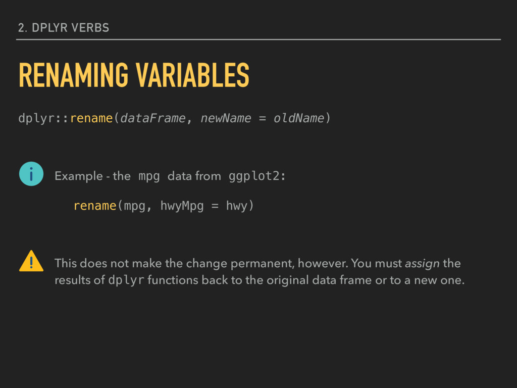
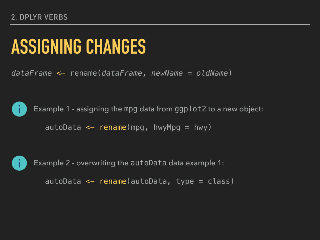
ggplot2: rename(mpg, hwyMpg = hwy) This does not make the change permanent, however. You must assign the results of dplyr functions back to the original data frame or to a new one. 2. DPLYR VERBS RENAMING VARIABLES
the mpg data from ggplot2 to a new object: autoData <- rename(mpg, hwyMpg = hwy) Example 2 - overwriting the autoData data example 1: autoData <- rename(autoData, type = class) 2. DPLYR VERBS ASSIGNING CHANGES
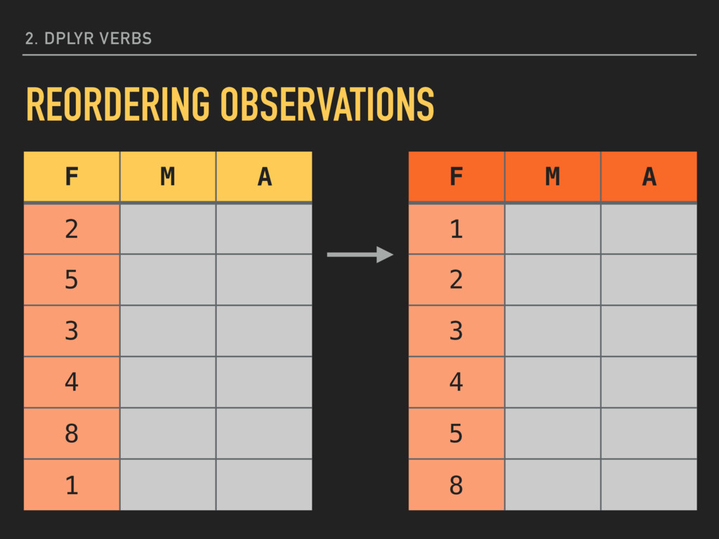
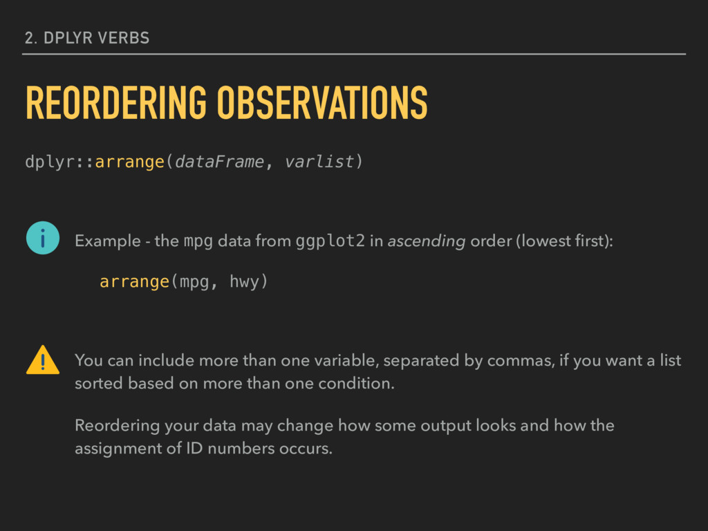
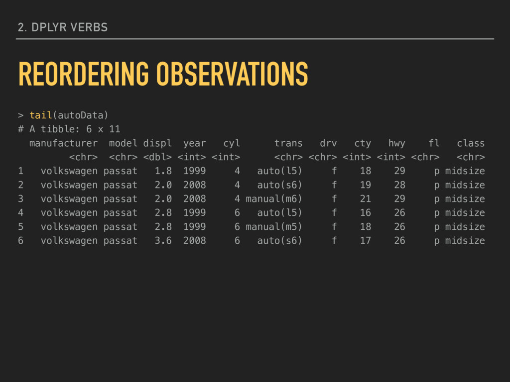
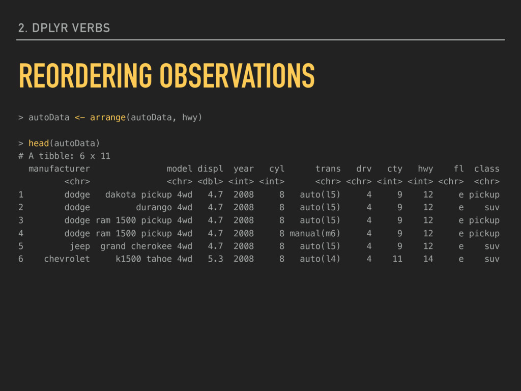
ascending order (lowest first): arrange(mpg, hwy) You can include more than one variable, separated by commas, if you want a list sorted based on more than one condition. Reordering your data may change how some output looks and how the assignment of ID numbers occurs. 2. DPLYR VERBS REORDERING OBSERVATIONS
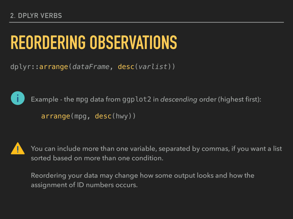
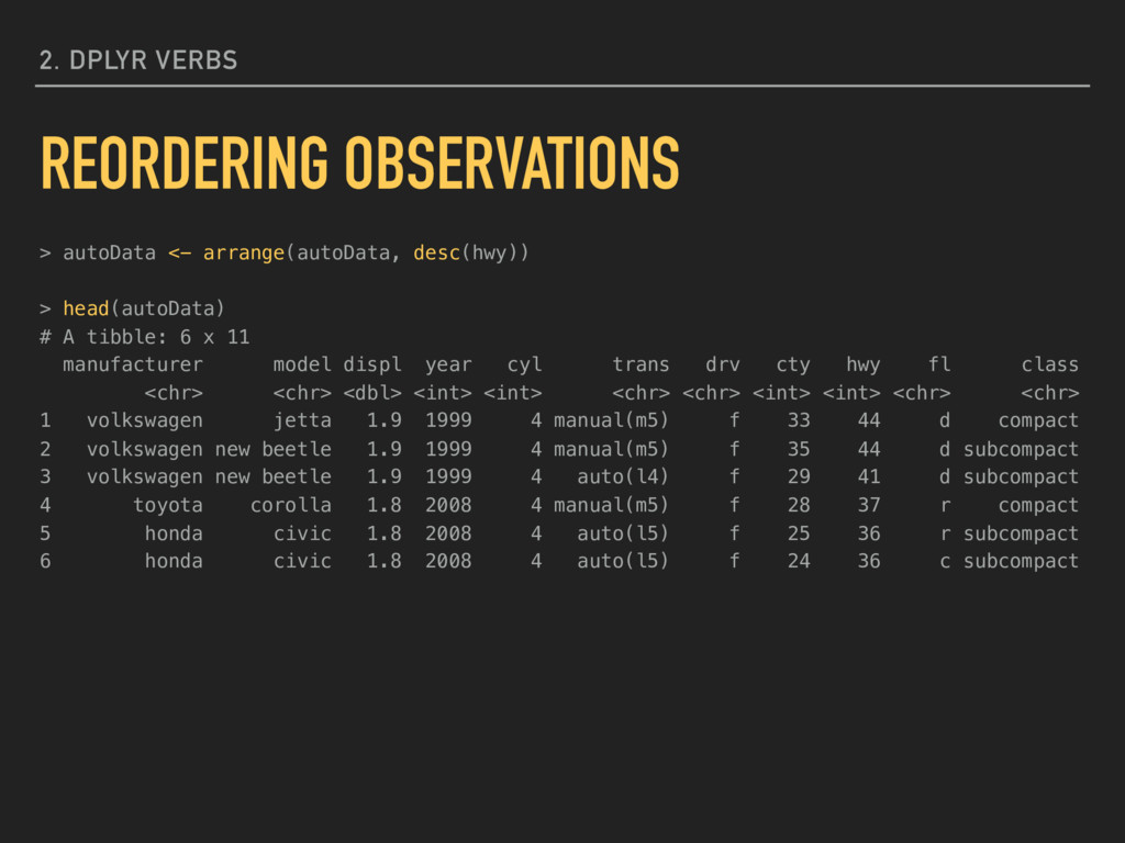
descending order (highest first): arrange(mpg, desc(hwy)) You can include more than one variable, separated by commas, if you want a list sorted based on more than one condition. Reordering your data may change how some output looks and how the assignment of ID numbers occurs. 2. DPLYR VERBS REORDERING OBSERVATIONS
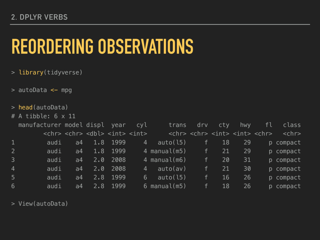
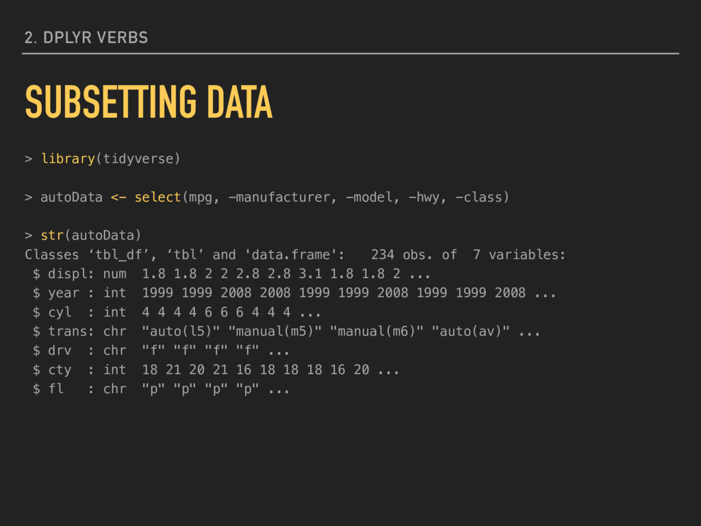
mpg > head(autoData) # A tibble: 6 x 11 manufacturer model displ year cyl trans drv cty hwy fl class <chr> <chr> <dbl> <int> <int> <chr> <chr> <int> <int> <chr> <chr> 1 audi a4 1.8 1999 4 auto(l5) f 18 29 p compact 2 audi a4 1.8 1999 4 manual(m5) f 21 29 p compact 3 audi a4 2.0 2008 4 manual(m6) f 20 31 p compact 4 audi a4 2.0 2008 4 auto(av) f 21 30 p compact 5 audi a4 2.8 1999 6 auto(l5) f 16 26 p compact 6 audi a4 2.8 1999 6 manual(m5) f 18 26 p compact > View(autoData)
> head(autoData) # A tibble: 6 x 11 manufacturer model displ year cyl trans drv cty hwy fl class <chr> <chr> <dbl> <int> <int> <chr> <chr> <int> <int> <chr> <chr> 1 volkswagen jetta 1.9 1999 4 manual(m5) f 33 44 d compact 2 volkswagen new beetle 1.9 1999 4 manual(m5) f 35 44 d subcompact 3 volkswagen new beetle 1.9 1999 4 auto(l4) f 29 41 d subcompact 4 toyota corolla 1.8 2008 4 manual(m5) f 28 37 r compact 5 honda civic 1.8 2008 4 auto(l5) f 25 36 r subcompact 6 honda civic 1.8 2008 4 auto(l5) f 24 36 c subcompact
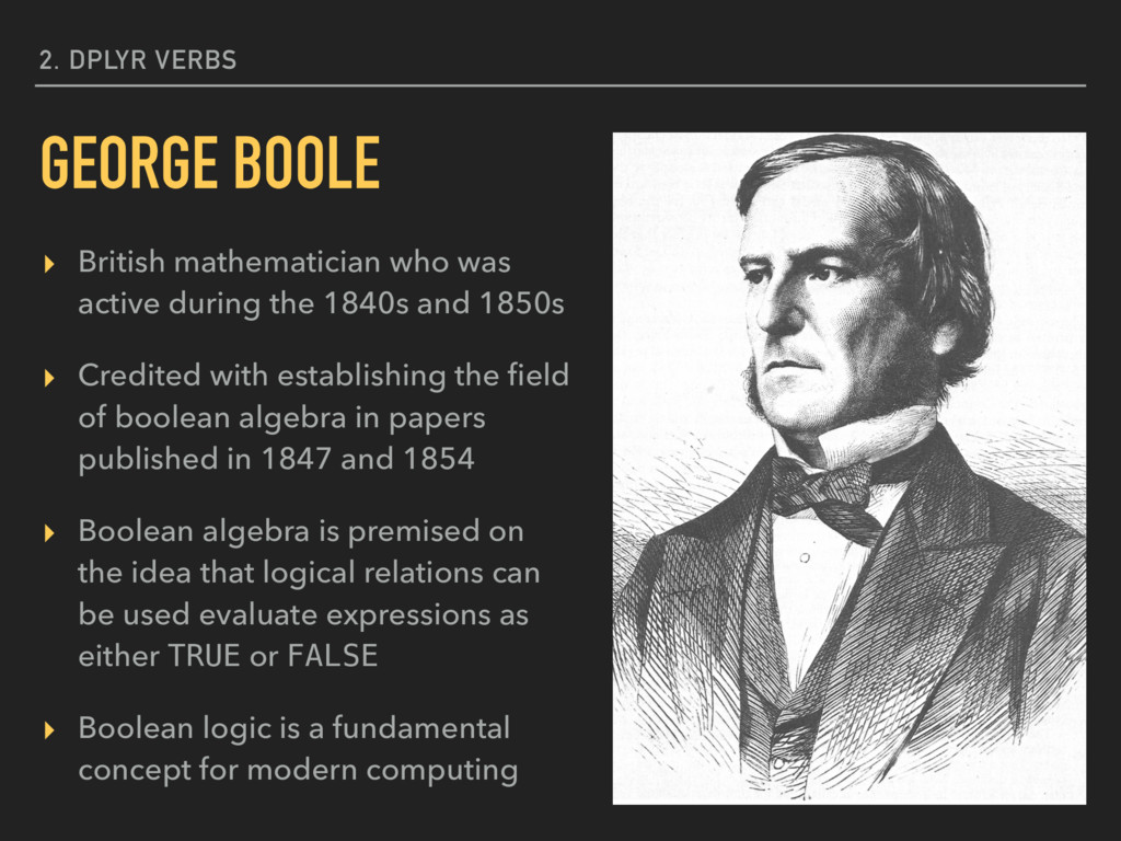
the 1840s and 1850s ▸ Credited with establishing the field of boolean algebra in papers published in 1847 and 1854 ▸ Boolean algebra is premised on the idea that logical relations can be used evaluate expressions as either TRUE or FALSE ▸ Boolean logic is a fundamental concept for modern computing GEORGE BOOLE
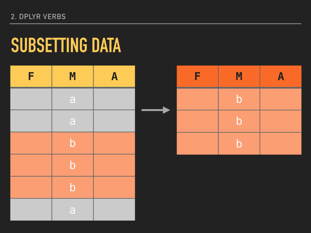
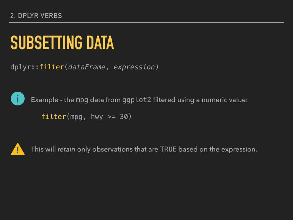
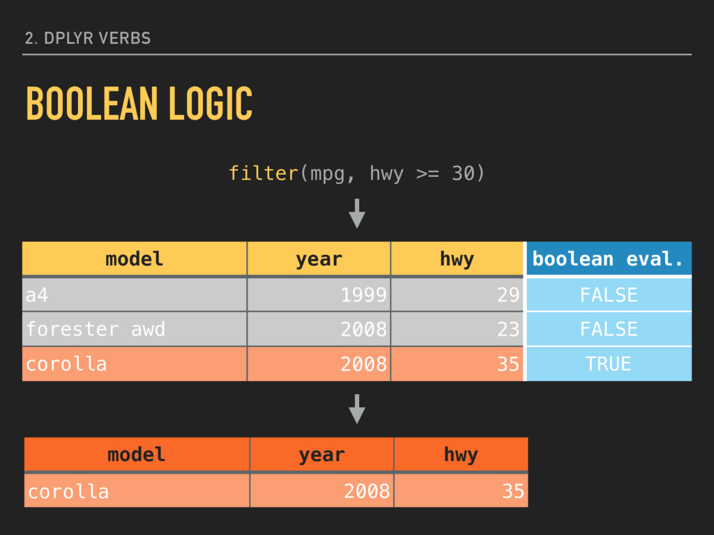
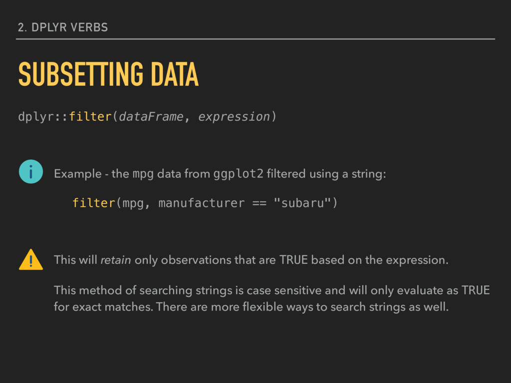
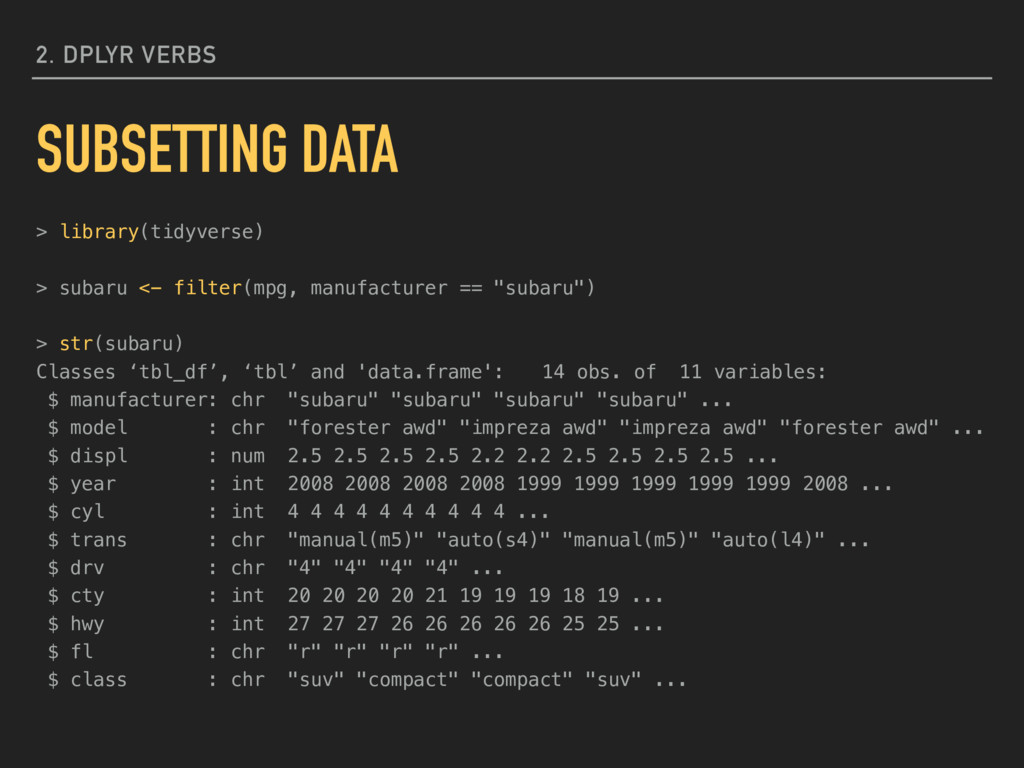
using a string: filter(mpg, manufacturer == "subaru") This will retain only observations that are TRUE based on the expression. This method of searching strings is case sensitive and will only evaluate as TRUE for exact matches. There are more flexible ways to search strings as well. 2. DPLYR VERBS SUBSETTING DATA
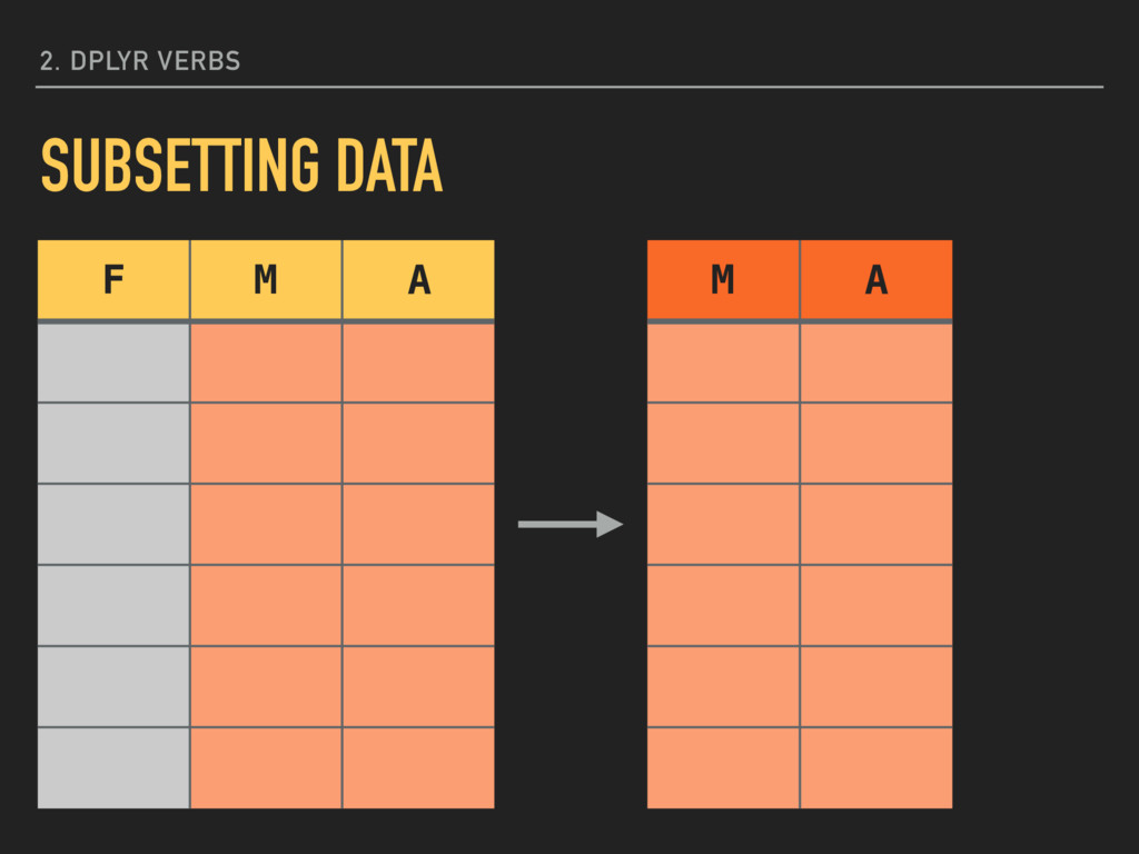
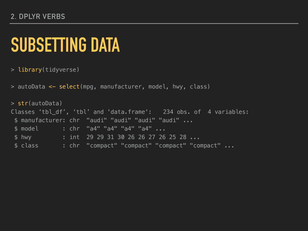
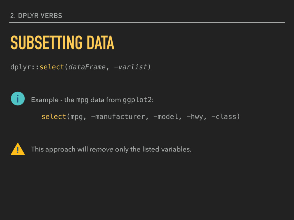
manufacturer, model, hwy, class) This approach will retain only the listed variables. There are additional helper functions for searching 2. DPLYR VERBS SUBSETTING DATA
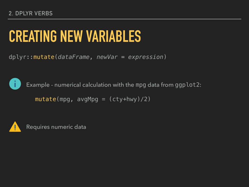
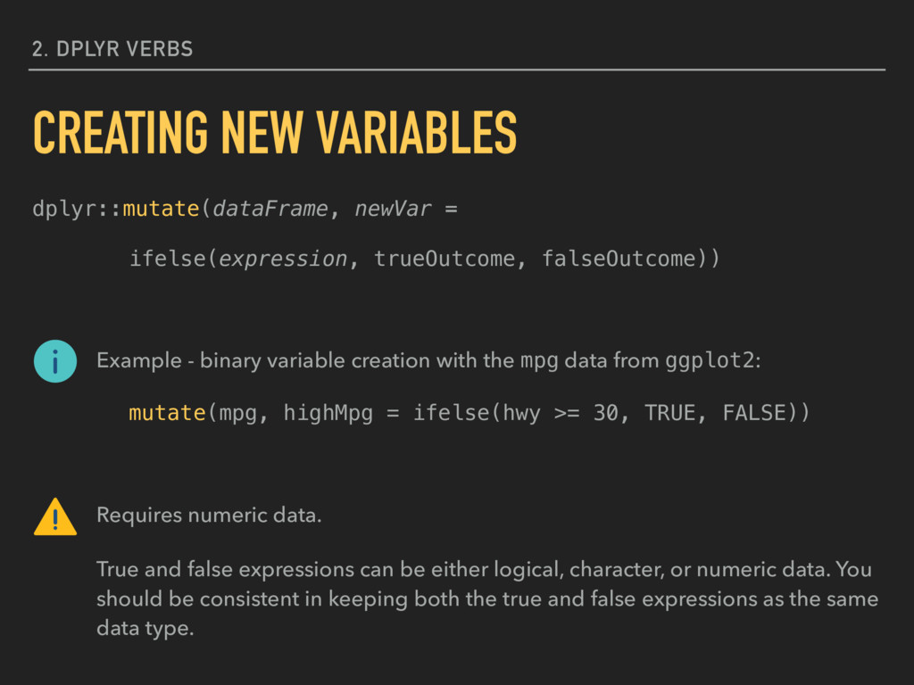
creation with the mpg data from ggplot2: mutate(mpg, highMpg = ifelse(hwy >= 30, TRUE, FALSE)) Requires numeric data. True and false expressions can be either logical, character, or numeric data. You should be consistent in keeping both the true and false expressions as the same data type. 2. DPLYR VERBS CREATING NEW VARIABLES
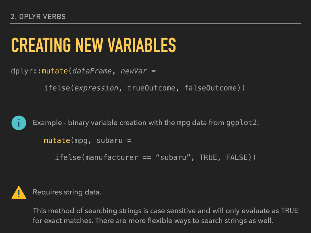
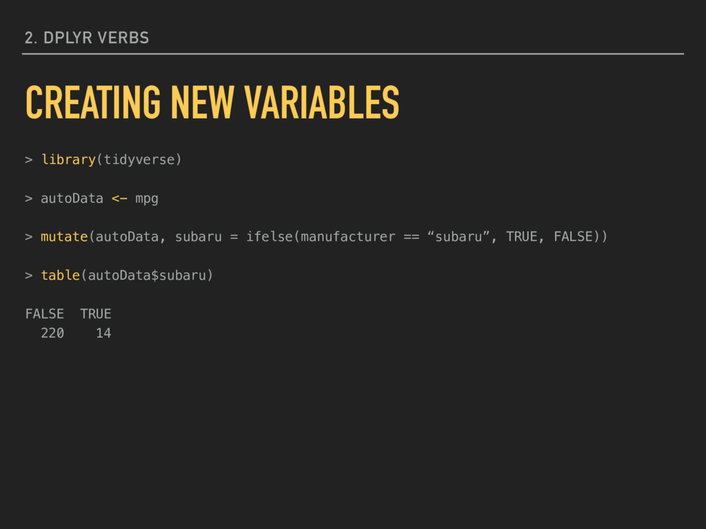
creation with the mpg data from ggplot2: mutate(mpg, subaru = ifelse(manufacturer == “subaru”, TRUE, FALSE)) Requires string data. This method of searching strings is case sensitive and will only evaluate as TRUE for exact matches. There are more flexible ways to search strings as well. 2. DPLYR VERBS CREATING NEW VARIABLES
PROGRAMS: INSTEAD OF IMAGINING THAT OUR MAIN TASK IS TO INSTRUCT A COMPUTER WHAT TO DO, LET US CONCENTRATE RATHER ON EXPLAINING TO HUMANS WHAT WE WANT THE COMPUTER TO DO. Donald E. Knuth Stanford University Computer Scientist
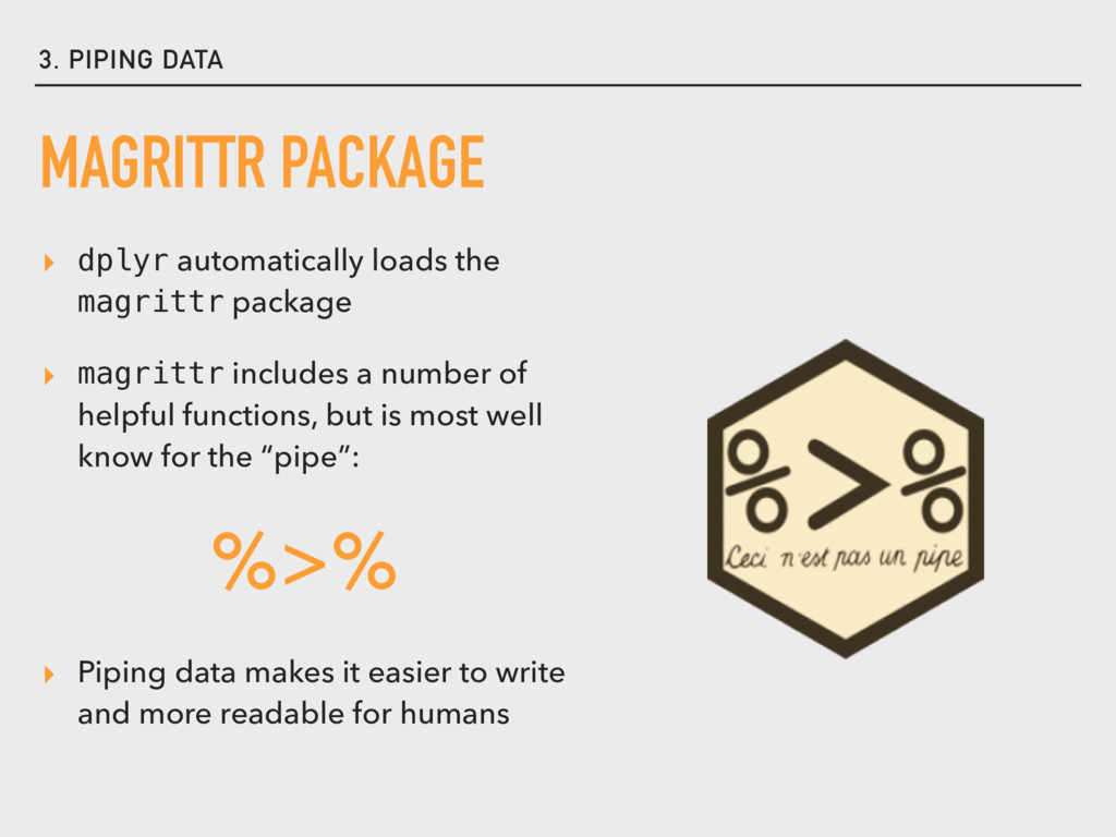
▸ magrittr includes a number of helpful functions, but is most well know for the “pipe”: ▸ Piping data makes it easier to write and more readable for humans MAGRITTR PACKAGE %>%
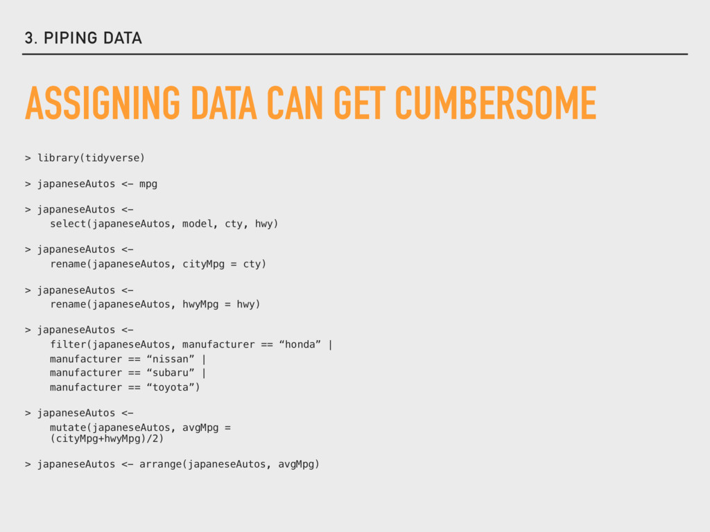
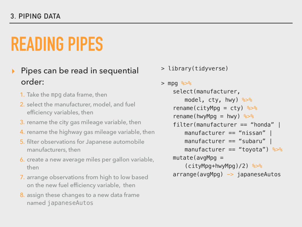
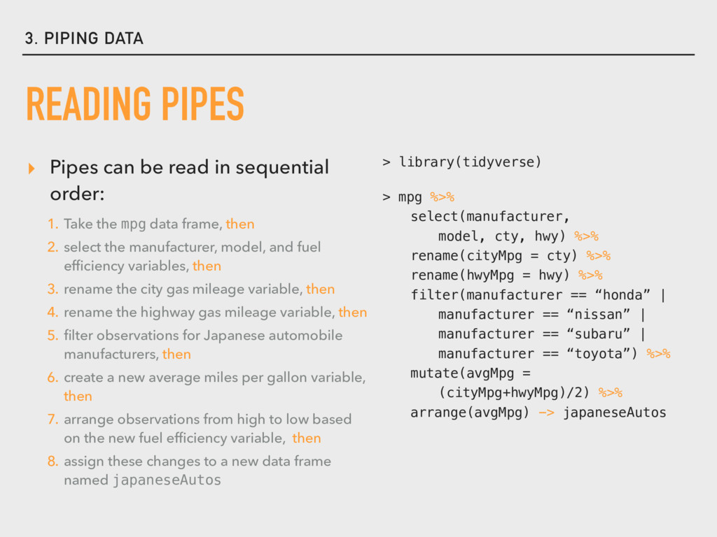
order: READING PIPES > library(tidyverse) > mpg %>% select(manufacturer, model, cty, hwy) %>% rename(cityMpg = cty) %>% rename(hwyMpg = hwy) %>% filter(manufacturer == “honda” | manufacturer == “nissan” | manufacturer == “subaru” | manufacturer == “toyota”) %>% mutate(avgMpg = (cityMpg+hwyMpg)/2) %>% arrange(avgMpg) -> japaneseAutos 1. Take the mpg data frame, then 2. select the manufacturer, model, and fuel efficiency variables, then 3. rename the city gas mileage variable, then 4. rename the highway gas mileage variable, then 5. filter observations for Japanese automobile manufacturers, then 6. create a new average miles per gallon variable, then 7. arrange observations from high to low based on the new fuel efficiency variable, then 8. assign these changes to a new data frame named japaneseAutos
order: READING PIPES > library(tidyverse) > mpg %>% select(manufacturer, model, cty, hwy) %>% rename(cityMpg = cty) %>% rename(hwyMpg = hwy) %>% filter(manufacturer == “honda” | manufacturer == “nissan” | manufacturer == “subaru” | manufacturer == “toyota”) %>% mutate(avgMpg = (cityMpg+hwyMpg)/2) %>% arrange(avgMpg) -> japaneseAutos 1. Take the mpg data frame, then 2. select the manufacturer, model, and fuel efficiency variables, then 3. rename the city gas mileage variable, then 4. rename the highway gas mileage variable, then 5. filter observations for Japanese automobile manufacturers, then 6. create a new average miles per gallon variable, then 7. arrange observations from high to low based on the new fuel efficiency variable, then 8. assign these changes to a new data frame named japaneseAutos
made on the first line of code like the example to the right ▸ I prefer the initial method only because the code “reads” in a linear fashion ▸ In either case, the data reference in each function can be omitted since it is “passed” by the pipe operator ▸ Pipes should be short READING PIPES > library(tidyverse) > japaneseAutos <- mpg %>% select(manufacturer, model, cty, hwy) %>% rename(cityMpg = cty) %>% rename(hwyMpg = hwy) %>% filter(manufacturer == “honda” | manufacturer == “nissan” | manufacturer == “subaru” | manufacturer == “toyota”) %>% mutate(avgMpg = (cityMpg+hwyMpg)/2) %>% arrange(avgMpg)
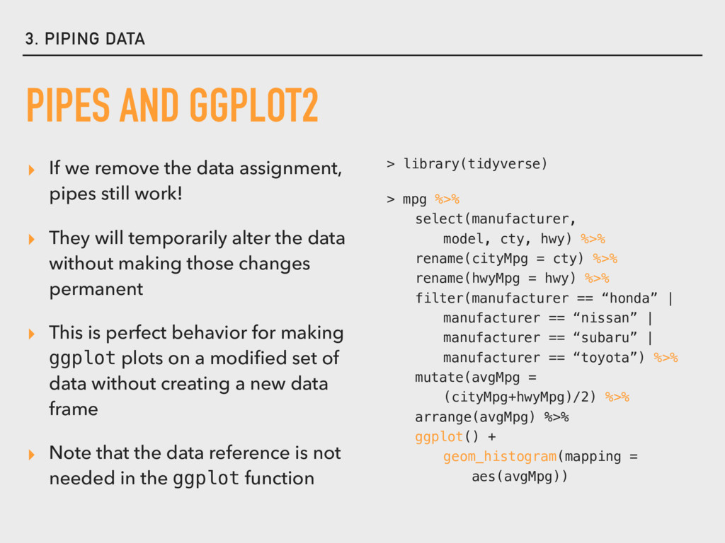
pipes still work! ▸ They will temporarily alter the data without making those changes permanent ▸ This is perfect behavior for making ggplot plots on a modified set of data without creating a new data frame ▸ Note that the data reference is not needed in the ggplot function PIPES AND GGPLOT2 > library(tidyverse) > mpg %>% select(manufacturer, model, cty, hwy) %>% rename(cityMpg = cty) %>% rename(hwyMpg = hwy) %>% filter(manufacturer == “honda” | manufacturer == “nissan” | manufacturer == “subaru” | manufacturer == “toyota”) %>% mutate(avgMpg = (cityMpg+hwyMpg)/2) %>% arrange(avgMpg) %>% ggplot() + geom_histogram(mapping = aes(avgMpg))