An MCMC for Supernovae Data

Talk for our MACSS project

Transcript

1. An MCMC for SNe Data Group 4 Juan Carlos Hidalgo Josué de Santiago MACCS April 21, 2016 . . . . . . . . . . . . . . . . . . . .
2. . . . . . . . . . . . . . . . . . . . . . . . . . . . . . . . . . . . . . . . . | Quiz An MCMC for SNe Data 2/1
3. . . . . . . . . . . . . . . . . . . . . . . . . . . . . . . . . . . . . . . . . | Quiz Which of the following would be brighter, in terms of the amount of energy delivered to your retina: An MCMC for SNe Data 2/1
4. . . . . . . . . . . . . . . . . . . . . . . . . . . . . . . . . . . . . . . . . | Quiz Which of the following would be brighter, in terms of the amount of energy delivered to your retina: A supernova, seen from as far away as the Sun is from the Earth, or The detonation of a hydrogen bomb pressed against your eyeball? An MCMC for SNe Data 2/1
5. . . . . . . . . . . . . . . . . . . . . . . . . . . . . . . . . . . . . . . . . | Quiz Which of the following would be brighter, in terms of the amount of energy delivered to your retina: A supernova, seen from as far away as the Sun is from the Earth, or The detonation of a hydrogen bomb pressed against your eyeball? An MCMC for SNe Data 2/1
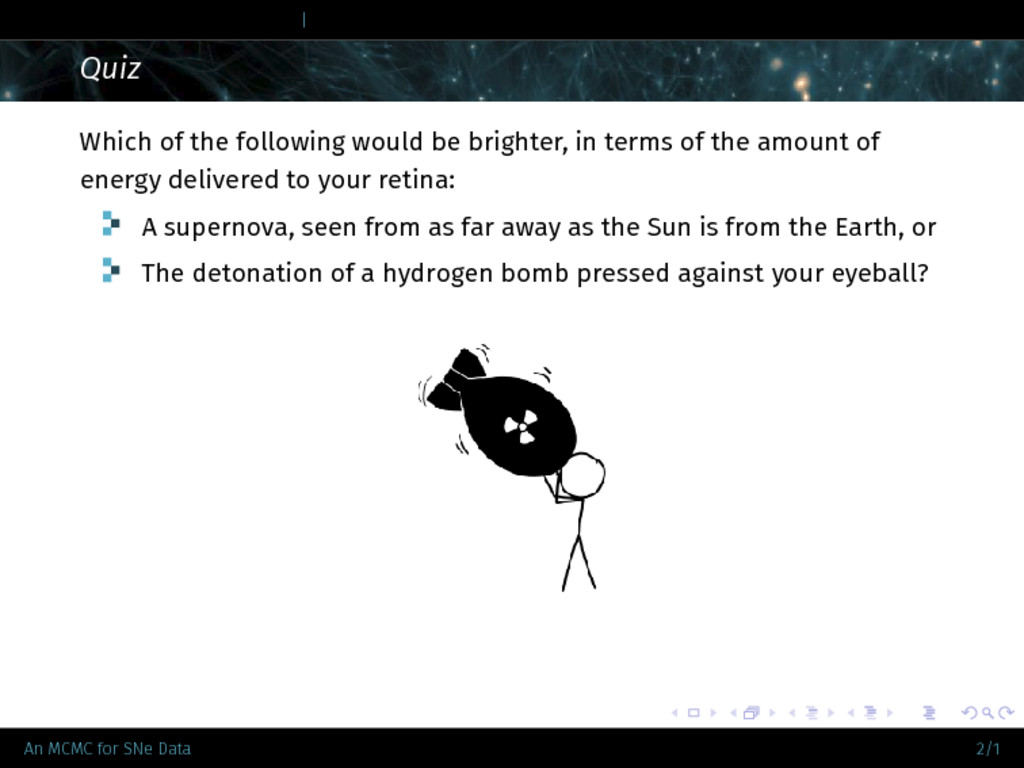
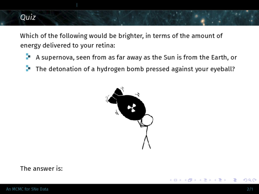
6. . . . . . . . . . . . . . . . . . . . . . . . . . . . . . . . . . . . . . . . . | Quiz Which of the following would be brighter, in terms of the amount of energy delivered to your retina: A supernova, seen from as far away as the Sun is from the Earth, or The detonation of a hydrogen bomb pressed against your eyeball? The answer is: An MCMC for SNe Data 2/1
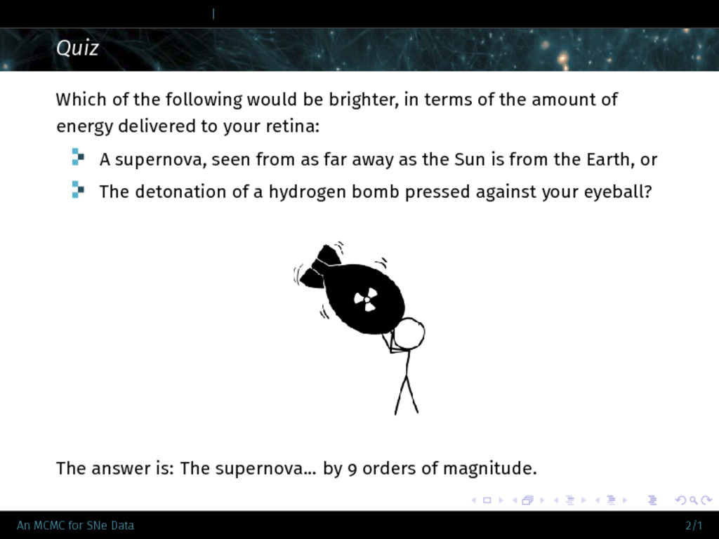
7. . . . . . . . . . . . . . . . . . . . . . . . . . . . . . . . . . . . . . . . . | Quiz Which of the following would be brighter, in terms of the amount of energy delivered to your retina: A supernova, seen from as far away as the Sun is from the Earth, or The detonation of a hydrogen bomb pressed against your eyeball? The answer is: The supernova... by 9 orders of magnitude. An MCMC for SNe Data 2/1
8. Introduction . . . . . . . . . . . . . . . . . . . .
9. . . . . . . . . . . . . . . . . . . . . . . . . . . . . . . . . . . . . . . . . | Objectives An MCMC for SNe Data 4/1
10. . . . . . . . . . . . . . . . . . . . . . . . . . . . . . . . . . . . . . . . . | Objectives Use the luminosity and redshift of Supernovae 1a events to infer cosmological parameters An MCMC for SNe Data 4/1
11. . . . . . . . . . . . . . . . . . . . . . . . . . . . . . . . . . . . . . . . . | Objectives Use the luminosity and redshift of Supernovae 1a events to infer cosmological parameters Compute the Likelihood and Posterior An MCMC for SNe Data 4/1
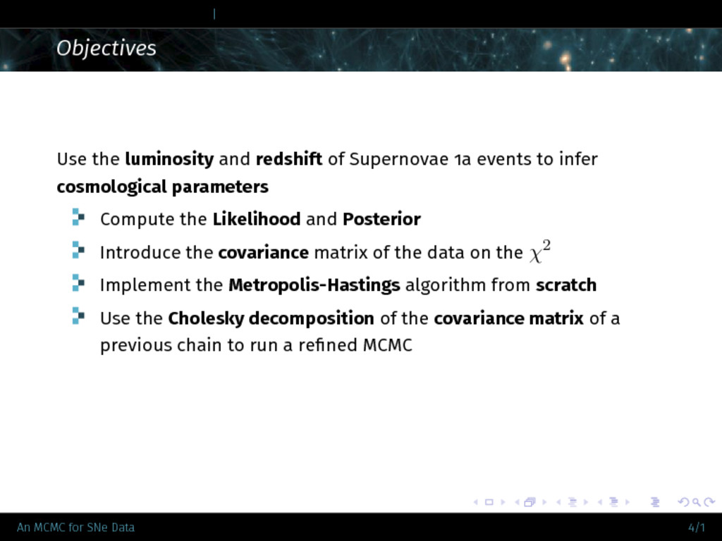
12. . . . . . . . . . . . . . . . . . . . . . . . . . . . . . . . . . . . . . . . . | Objectives Use the luminosity and redshift of Supernovae 1a events to infer cosmological parameters Compute the Likelihood and Posterior Introduce the covariance matrix of the data on the χ2 An MCMC for SNe Data 4/1
13. . . . . . . . . . . . . . . . . . . . . . . . . . . . . . . . . . . . . . . . . | Objectives Use the luminosity and redshift of Supernovae 1a events to infer cosmological parameters Compute the Likelihood and Posterior Introduce the covariance matrix of the data on the χ2 Implement the Metropolis-Hastings algorithm from scratch An MCMC for SNe Data 4/1
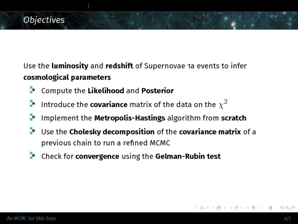
14. . . . . . . . . . . . . . . . . . . . . . . . . . . . . . . . . . . . . . . . . | Objectives Use the luminosity and redshift of Supernovae 1a events to infer cosmological parameters Compute the Likelihood and Posterior Introduce the covariance matrix of the data on the χ2 Implement the Metropolis-Hastings algorithm from scratch Use the Cholesky decomposition of the covariance matrix of a previous chain to run a refined MCMC An MCMC for SNe Data 4/1
15. . . . . . . . . . . . . . . . . . . . . . . . . . . . . . . . . . . . . . . . . | Objectives Use the luminosity and redshift of Supernovae 1a events to infer cosmological parameters Compute the Likelihood and Posterior Introduce the covariance matrix of the data on the χ2 Implement the Metropolis-Hastings algorithm from scratch Use the Cholesky decomposition of the covariance matrix of a previous chain to run a refined MCMC Check for convergence using the Gelman-Rubin test An MCMC for SNe Data 4/1
16. . . . . . . . . . . . . . . . . . . . . . . . . . . . . . . . . . . . . . . . . | The Model On a flat universe d ℓ(z, h, ΩΛ) = (1 + z)c 100h Km s·Mpc ∫ z 0 dz √ (1 − ΩΛ)(1 + z)3 + ΩΛ All supernovae 1a events have a luminosity module given by µth(z, h, ΩΛ) = 5 log 10 (d ℓ(z, h, ΩΛ)) + 25 An MCMC for SNe Data 5/1
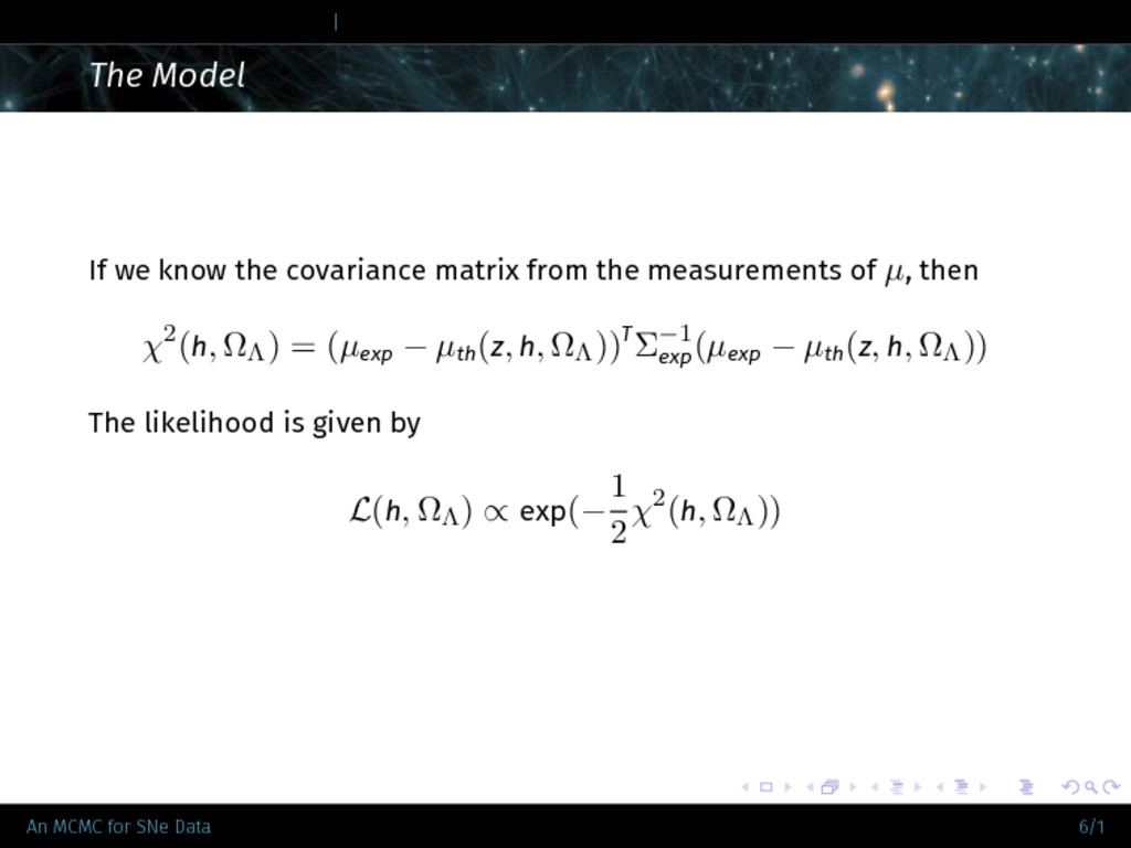
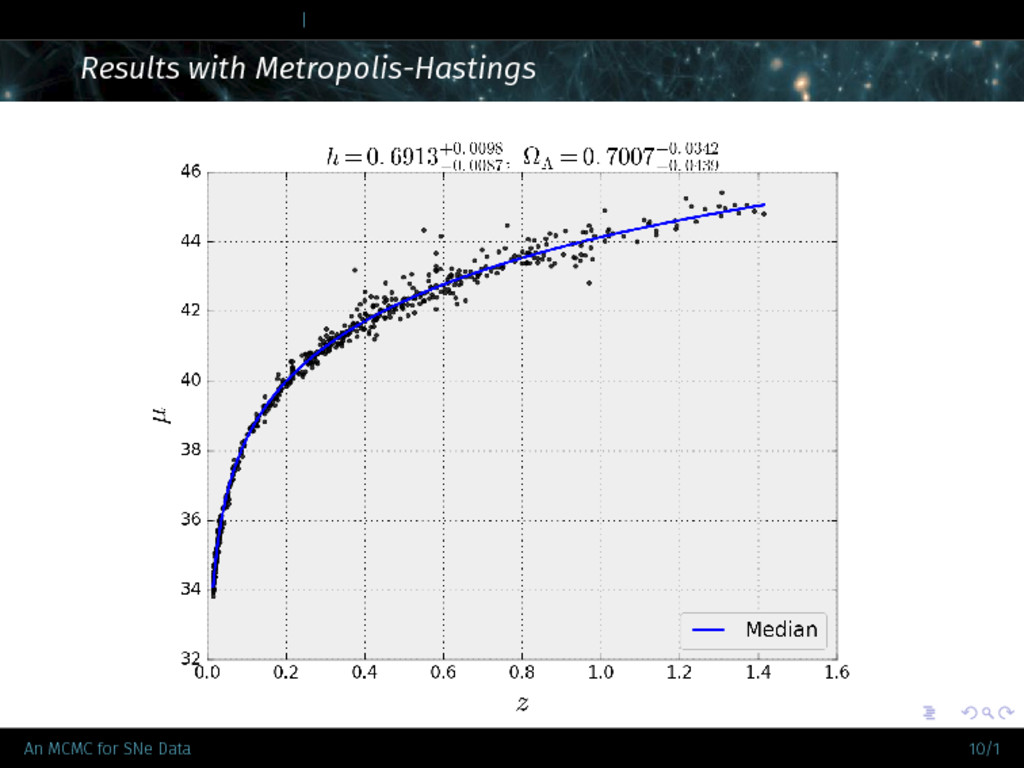
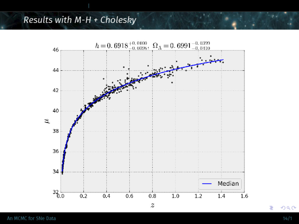
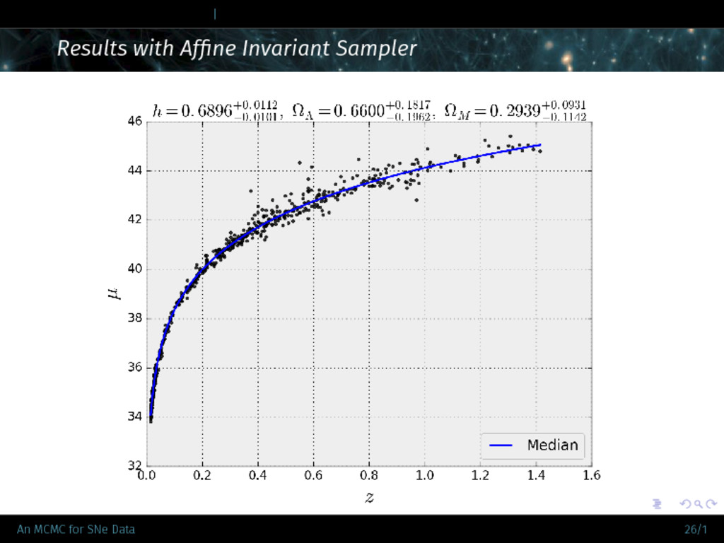
17. . . . . . . . . . . . . . . . . . . . . . . . . . . . . . . . . . . . . . . . . | The Model If we know the covariance matrix from the measurements of µ, then χ2(h, ΩΛ) = (µexp − µth(z, h, ΩΛ))T Σ−1 exp (µexp − µth(z, h, ΩΛ)) The likelihood is given by L(h, ΩΛ) ∝ exp(− 1 2 χ2(h, ΩΛ)) An MCMC for SNe Data 6/1
18. Metropolis-Hastings from Scratch . . . . . . . . . . . . . . . . . . . .
19. . . . . . . . . . . . . . . . . . . . . . . . . . . . . . . . . . . . . . . . . | Metropolis-Hastings Algorithm An MCMC for SNe Data 8/1
20. . . . . . . . . . . . . . . . . . . . . . . . . . . . . . . . . . . . . . . . . | Metropolis-Hastings Algorithm Step 1: Pick a point to start the walk (h 0, Ω0) An MCMC for SNe Data 8/1
21. . . . . . . . . . . . . . . . . . . . . . . . . . . . . . . . . . . . . . . . . | Metropolis-Hastings Algorithm Step 1: Pick a point to start the walk (h 0, Ω0) Step 2: Update the point (hi, Ωi) hi+1 = hi + N(0, 1) Ωi+1 = Ωi + N(0, 1) An MCMC for SNe Data 8/1
22. . . . . . . . . . . . . . . . . . . . . . . . . . . . . . . . . . . . . . . . . | Metropolis-Hastings Algorithm Step 1: Pick a point to start the walk (h 0, Ω0) Step 2: Update the point (hi, Ωi) hi+1 = hi + N(0, 1) Ωi+1 = Ωi + N(0, 1) Step 3: Compute the logarithm of the ratio of Likelihoods r = 1 2 χ2(hi, Ωi) − 1 2 χ2(hi+1, Ωi+1) An MCMC for SNe Data 8/1
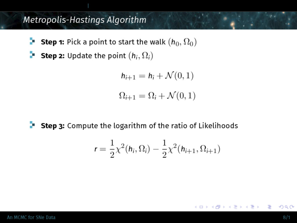
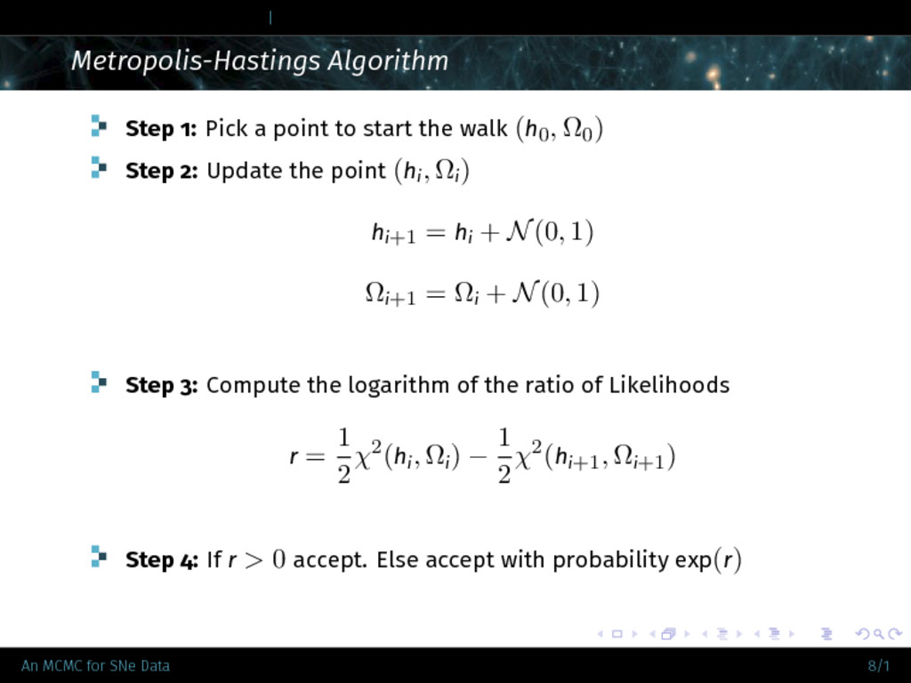
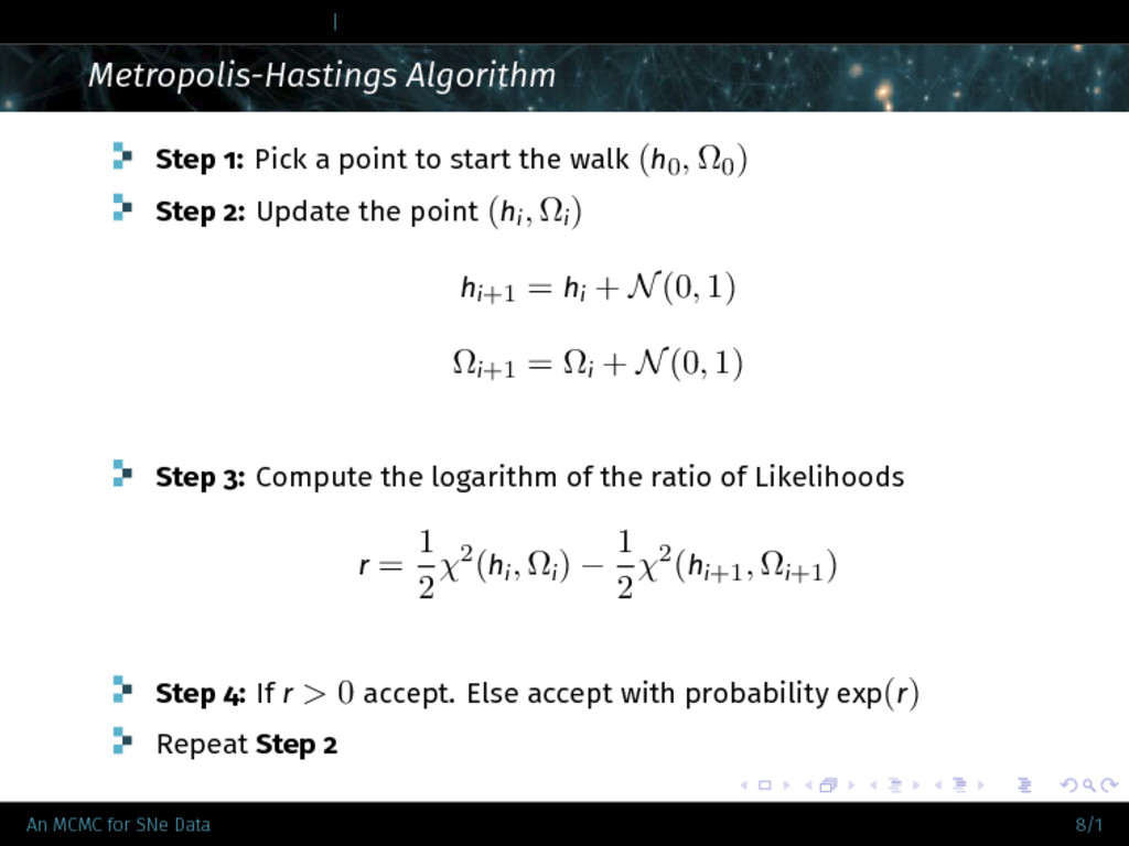
23. . . . . . . . . . . . . . . . . . . . . . . . . . . . . . . . . . . . . . . . . | Metropolis-Hastings Algorithm Step 1: Pick a point to start the walk (h 0, Ω0) Step 2: Update the point (hi, Ωi) hi+1 = hi + N(0, 1) Ωi+1 = Ωi + N(0, 1) Step 3: Compute the logarithm of the ratio of Likelihoods r = 1 2 χ2(hi, Ωi) − 1 2 χ2(hi+1, Ωi+1) Step 4: If r > 0 accept. Else accept with probability exp(r) An MCMC for SNe Data 8/1
24. . . . . . . . . . . . . . . . . . . . . . . . . . . . . . . . . . . . . . . . . | Metropolis-Hastings Algorithm Step 1: Pick a point to start the walk (h 0, Ω0) Step 2: Update the point (hi, Ωi) hi+1 = hi + N(0, 1) Ωi+1 = Ωi + N(0, 1) Step 3: Compute the logarithm of the ratio of Likelihoods r = 1 2 χ2(hi, Ωi) − 1 2 χ2(hi+1, Ωi+1) Step 4: If r > 0 accept. Else accept with probability exp(r) Repeat Step 2 An MCMC for SNe Data 8/1
25. . . . . . . . . . . . . . . . . . . . . . . . . . . . . . . . . . . . . . . . . | Results with Metropolis-Hastings An MCMC for SNe Data 9/1
26. . . . . . . . . . . . . . . . . . . . . . . . . . . . . . . . . . . . . . . . . | Results with Metropolis-Hastings An MCMC for SNe Data 10/1
27. Refining Metropolis-Hastings . . . . . . . . . . . . . . . . . . . .
28. . . . . . . . . . . . . . . . . . . . . . . . . . . . . . . . . . . . . . . . . | Cholesky Decompostion An MCMC for SNe Data 12/1
29. . . . . . . . . . . . . . . . . . . . . . . . . . . . . . . . . . . . . . . . . | Cholesky Decompostion Let Σ be a Symmetric positive-definite matrix An MCMC for SNe Data 12/1
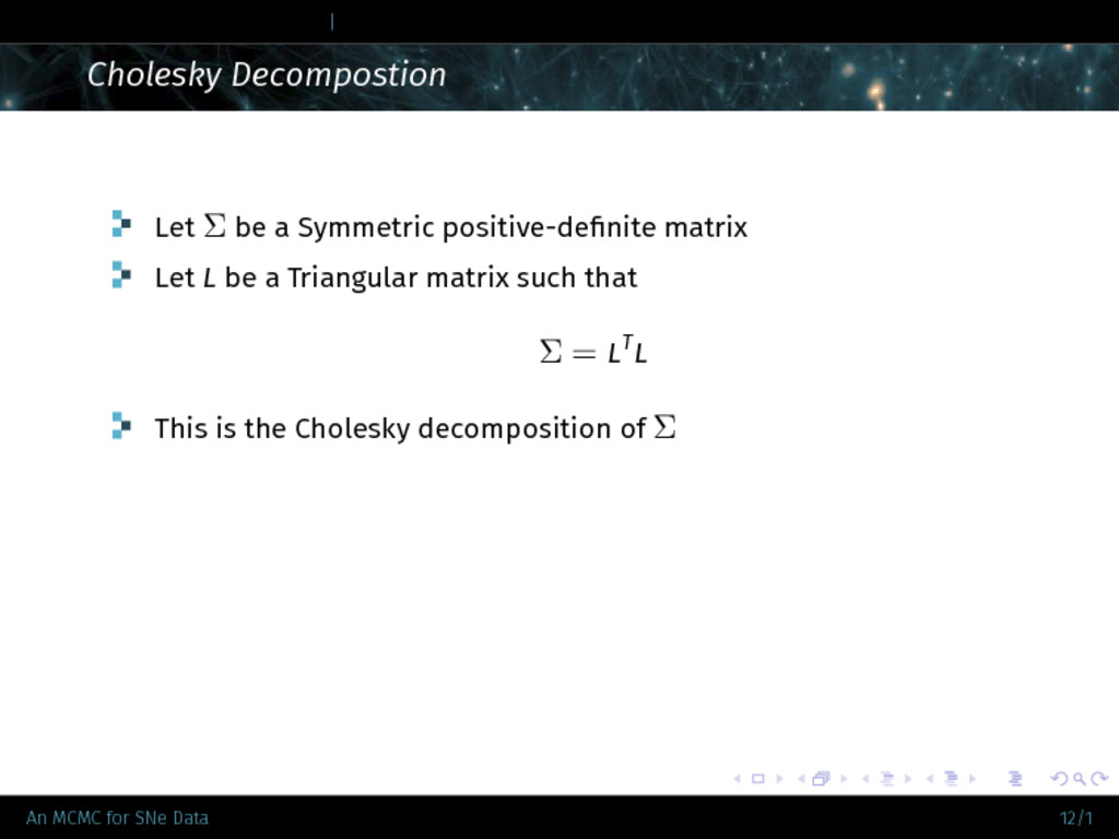
30. . . . . . . . . . . . . . . . . . . . . . . . . . . . . . . . . . . . . . . . . | Cholesky Decompostion Let Σ be a Symmetric positive-definite matrix Let L be a Triangular matrix such that Σ = LTL This is the Cholesky decomposition of Σ An MCMC for SNe Data 12/1
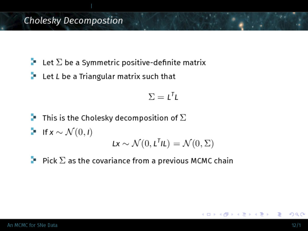
31. . . . . . . . . . . . . . . . . . . . . . . . . . . . . . . . . . . . . . . . . | Cholesky Decompostion Let Σ be a Symmetric positive-definite matrix Let L be a Triangular matrix such that Σ = LTL This is the Cholesky decomposition of Σ If x ∼ N(0, I) Lx ∼ N(0, LTIL) = N(0, Σ) Pick Σ as the covariance from a previous MCMC chain An MCMC for SNe Data 12/1
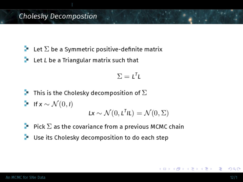
32. . . . . . . . . . . . . . . . . . . . . . . . . . . . . . . . . . . . . . . . . | Cholesky Decompostion Let Σ be a Symmetric positive-definite matrix Let L be a Triangular matrix such that Σ = LTL This is the Cholesky decomposition of Σ If x ∼ N(0, I) Lx ∼ N(0, LTIL) = N(0, Σ) Pick Σ as the covariance from a previous MCMC chain Use its Cholesky decomposition to do each step An MCMC for SNe Data 12/1
33. . . . . . . . . . . . . . . . . . . . . . . . . . . . . . . . . . . . . . . . . | Results with M-H + Cholesky An MCMC for SNe Data 13/1
34. . . . . . . . . . . . . . . . . . . . . . . . . . . . . . . . . . . . . . . . . | Results with M-H + Cholesky An MCMC for SNe Data 14/1
35. Checking Convergence . . . . . . . . . . . . . . . . . . . .
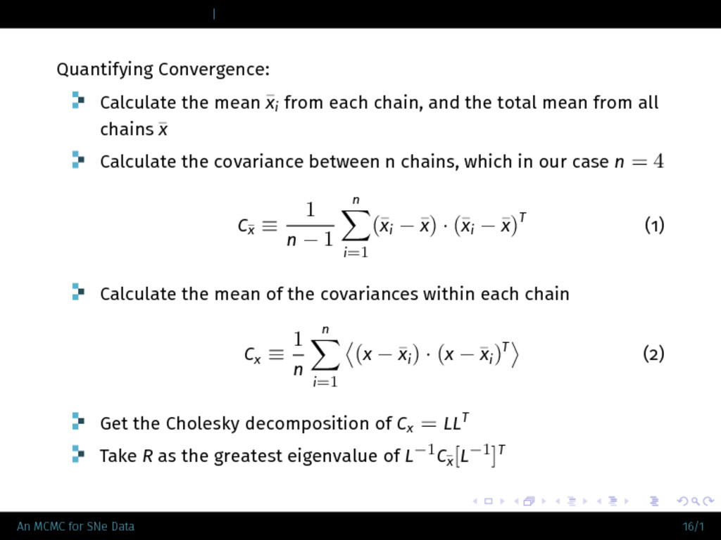
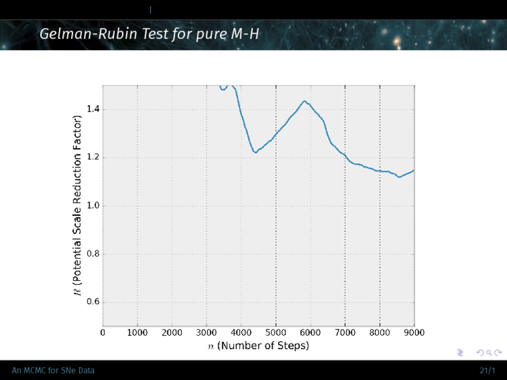
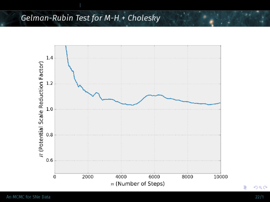
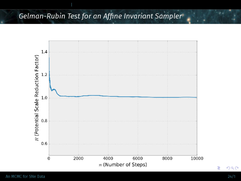
36. . . . . . . . . . . . . . . . . . . . . . . . . . . . . . . . . . . . . . . . . | Quantifying Convergence: Calculate the mean ¯ xi from each chain, and the total mean from all chains ¯ x Calculate the covariance between n chains, which in our case n = 4 C ¯ x ≡ 1 n − 1 n ∑ i=1 (¯ xi − ¯ x) · (¯ xi − ¯ x)T (1) Calculate the mean of the covariances within each chain Cx ≡ 1 n n ∑ i=1 ⟨ (x − ¯ xi) · (x − ¯ xi)T ⟩ (2) Get the Cholesky decomposition of Cx = LLT Take R as the greatest eigenvalue of L−1C ¯ x[L−1]T An MCMC for SNe Data 16/1
37. . . . . . . . . . . . . . . . . . . . . . . . . . . . . . . . . . . . . . . . . | Gelman-Rubin Test for pure M-H An MCMC for SNe Data 17/1
38. . . . . . . . . . . . . . . . . . . . . . . . . . . . . . . . . . . . . . . . . | Gelman-Rubin Test for M-H + Cholesky An MCMC for SNe Data 18/1
39. Non-Official Work . . . . . . . . . . . . . . . . . . . .
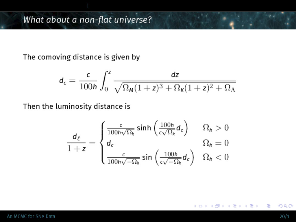
40. . . . . . . . . . . . . . . . . . . . . . . . . . . . . . . . . . . . . . . . . | What about a non-flat universe? The comoving distance is given by dc = c 100h ∫ z 0 dz √ ΩM(1 + z)3 + ΩK(1 + z)2 + ΩΛ Then the luminosity distance is d ℓ 1 + z =        c 100h √ Ωk sinh ( 100h c √ Ωk dc ) Ωk > 0 dc Ωk = 0 c 100h √ −Ωk sin ( 100h c √ −Ωk dc ) Ωk < 0 An MCMC for SNe Data 20/1
41. . . . . . . . . . . . . . . . . . . . . . . . . . . . . . . . . . . . . . . . . | Gelman-Rubin Test for pure M-H An MCMC for SNe Data 21/1
42. . . . . . . . . . . . . . . . . . . . . . . . . . . . . . . . . . . . . . . . . | Gelman-Rubin Test for M-H + Cholesky An MCMC for SNe Data 22/1
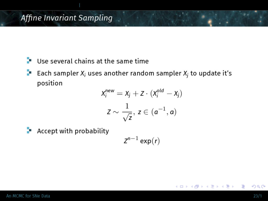
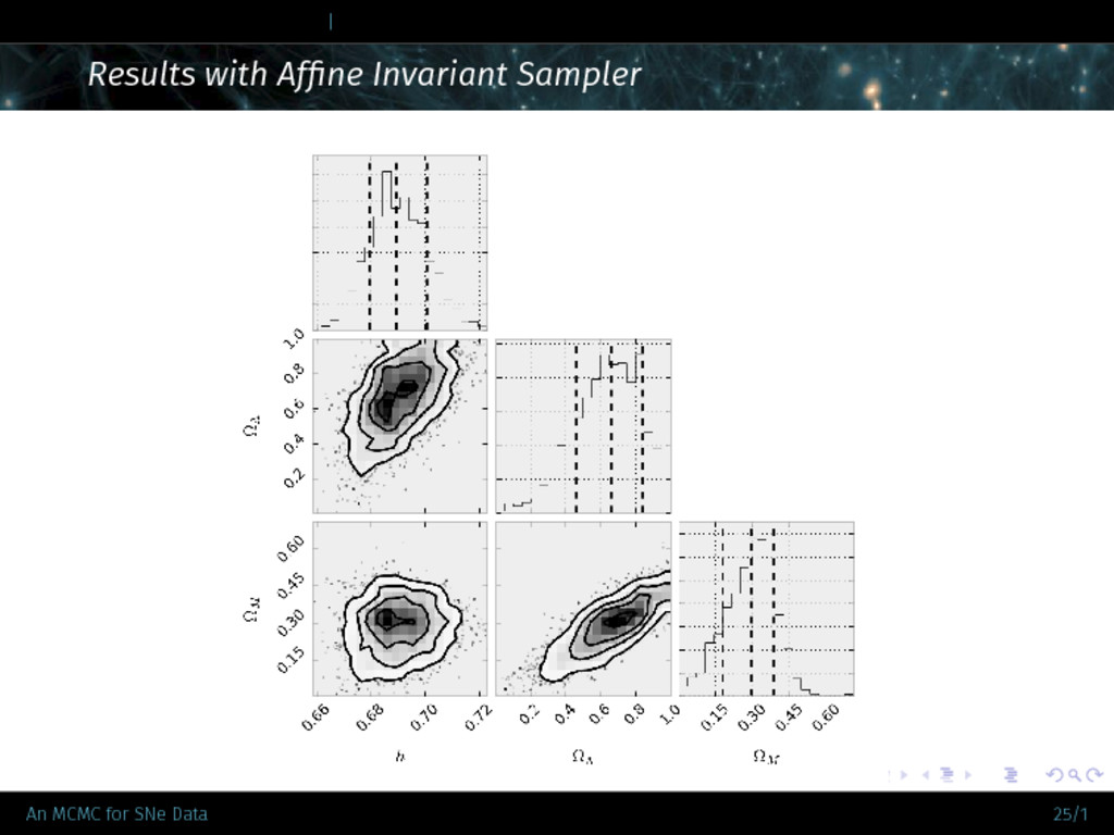
43. . . . . . . . . . . . . . . . . . . . . . . . . . . . . . . . . . . . . . . . . | Affine Invariant Sampling Use several chains at the same time Each sampler Xi uses another random sampler Xj to update it’s position Xnew i = Xj + Z · (Xold i − Xj) Z ∼ 1 √ z , z ∈ (a−1, a) Accept with probability Zn−1 exp(r) An MCMC for SNe Data 23/1
44. . . . . . . . . . . . . . . . . . . . . . . . . . . . . . . . . . . . . . . . . | Gelman-Rubin Test for an Affine Invariant Sampler An MCMC for SNe Data 24/1
45. . . . . . . . . . . . . . . . . . . . . . . . . . . . . . . . . . . . . . . . . | Results with Affine Invariant Sampler An MCMC for SNe Data 25/1
46. . . . . . . . . . . . . . . . . . . . . . . . . . . . . . . . . . . . . . . . . | Results with Affine Invariant Sampler An MCMC for SNe Data 26/1
47. . . . . . . . . . . . . . . . . . . . . . . . . . . . . . . . . . . . . . . . . | References Lewis, Antony. Efficient sampling of fast and slow cosmological parameters [v2] arXiv:1304.44. Goodman, Jonathan and Weare, Jonathan. Ensemble Samplers With Affine Invariance (2010). Communications in Applied Mathematics and Computational Science (vol. 5 no. 1) An MCMC for SNe Data 27/1