[Paper reading] Local Outlier Detection With Interpretation

This paper is published at ECML-PKDD 2013.
(http://www.ecmlpkdd2013.org/wp-content/uploads/2013/07/222.pdf)

Transcript

1. 1 KYOTO UNIVERSITY KYOTO UNIVERSITY Local Outlier Detection with Interpretation Daiki Tanaka Kashima lab., Kyoto University
2. 2 KYOTO UNIVERSITY Paper information: n Title : Local Outlier Detection with Interpretation n Venue : ECML-PKDD 2013 n Authors : l Xuan Hong Dang (Aarhus University, Denmark) l Barbora Micenkova (Aarhus University, Denmark) l Ira Assent (Aarhus University, Denmark) l Raymond T. Ng (University of British Columbia, Canada)
3. 3 KYOTO UNIVERSITY Background: Anomaly explanation has not been developed well. n Anomaly detection is important in many real world applications. n Although there are many techniques for discovering anomalous patterns, most attempts focus on the aspect of outlier identification, ignoring the outlier interpretation. n For many application domains, especially those with data described by a large number of features, the interpretation of outliers is essential. n Explanation offers people a facility to gain insights into why an outlier is exceptionally different from other regular objects.
4. 4 KYOTO UNIVERSITY Background: Global outliers and local outliers n Outlying patterns are divided into two types : global and local outliers. l A global outlier is an object which has a significantly large distance to its k-th nearest neighbor whereas a local outlier has a distance to its k-th neighbor that is large relatively to the average distance of its neighbors to their own k-th nearest neighbors. n The objective of this study is detecting and interpreting local outliers.
5. 5 KYOTO UNIVERSITY Related Work: There are not many studies that address outlier interpretation. n There are methods to find global outliers [E. M. Knorr+ 1998] [Y. Tao+ 2006] n Techniques relying on density attempt to seek local outliers whose anomaly degrees are defined by Local Outlier Factor. [M. M. Breunig+ 2000] n Recently, several studies that attempt to find outliers in subspace. [Z. He+ 2005][A. Foss+ 2009][F. Keller+ 2012] l Exploring subspace projection seems to be appropriate for outlier interpretation. n [E. M. Knorr+ 1999] was the only attempt that directly address issues of outlier interpretation. l But [E. M. Knorr+ 1999] was for global outliers.
6. 6 KYOTO UNIVERSITY Related Work: Recent studies n Several works aim to find an optimal feature subspace which distinguishes outliers from normal points to explain outliers. l Knorr, E.M et al. :Finding intensional knowledge of distance-based outliers. In: VLDB (1999) l Keller, F, et al. : Flexible and adaptive subspace search for outlier analysis. In: CIKM (2013) l Kuo, C.T, et al. : A framework for outlier description using constraint programming. In: AAAI (2016) l Micenkova, B, et al. : Explaining outliers by subspace separability. In: ICDM (2013) l Nikhil Gupta et al. : Beyond Outlier Detection: LookOut for Pictorial Explanation l N. Liu, et al. : Contextual outlier interpretation. In : IJICAI (2017)
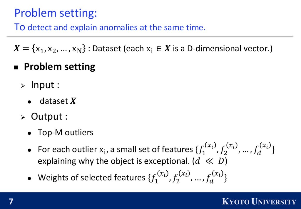
7. 7 KYOTO UNIVERSITY Problem setting: To detect and explain anomalies at the same time. ! = x$ , x& , … , x( : Dataset (each x) ∈ ! is a D-dimensional vector.) n Problem setting Ø Input : l dataset ! Ø Output : l Top-M outliers l For each outlier x) , a small set of features {, $ -. , , & -. , … , , / -. } explaining why the object is exceptional. (1 ≪ 3) l Weights of selected features {, $ -. , , & -. , … , , / -. }
8. 8 KYOTO UNIVERSITY Proposed Method : Overview There are three steps. n Local Outlier Detection with Interpretation (LODI) 1. Neighboring Set Selection 2. Anomaly Degree Computation 3. Outlier Interpretation
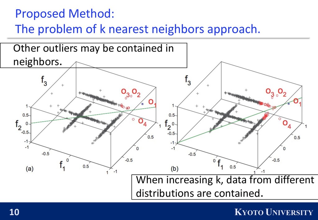
9. 9 KYOTO UNIVERSITY Proposed Method: 1.Neighboring Set Selection n Existing work uses k-nearest neighboring objects. l Deciding proper value of k is non-trivial task. l Such objects may contain nearby outliers or inliers from several distributions.
10. 10 KYOTO UNIVERSITY Proposed Method: The problem of k nearest neighbors approach. When increasing k, data from different distributions are contained. Other outliers may be contained in neighbors.
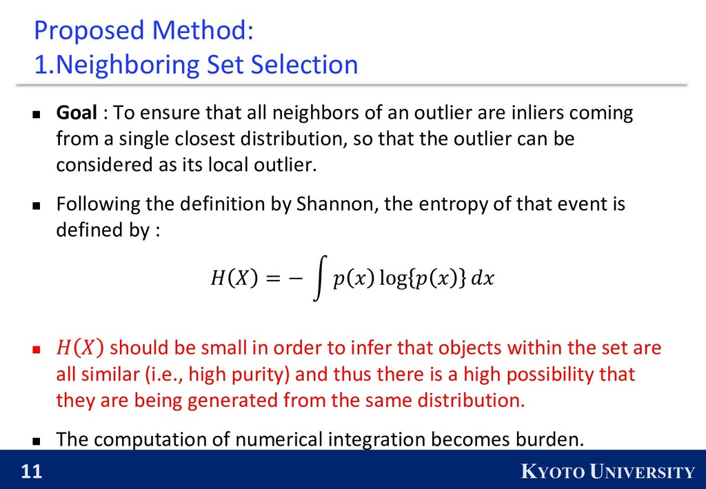
11. 11 KYOTO UNIVERSITY Proposed Method: 1.Neighboring Set Selection n Goal : To ensure that all neighbors of an outlier are inliers coming from a single closest distribution, so that the outlier can be considered as its local outlier. n Following the definition by Shannon, the entropy of that event is defined by : ! " = − % & ' log & ' +' n ! " should be small in order to infer that objects within the set are all similar (i.e., high purity) and thus there is a high possibility that they are being generated from the same distribution. n The computation of numerical integration becomes burden.
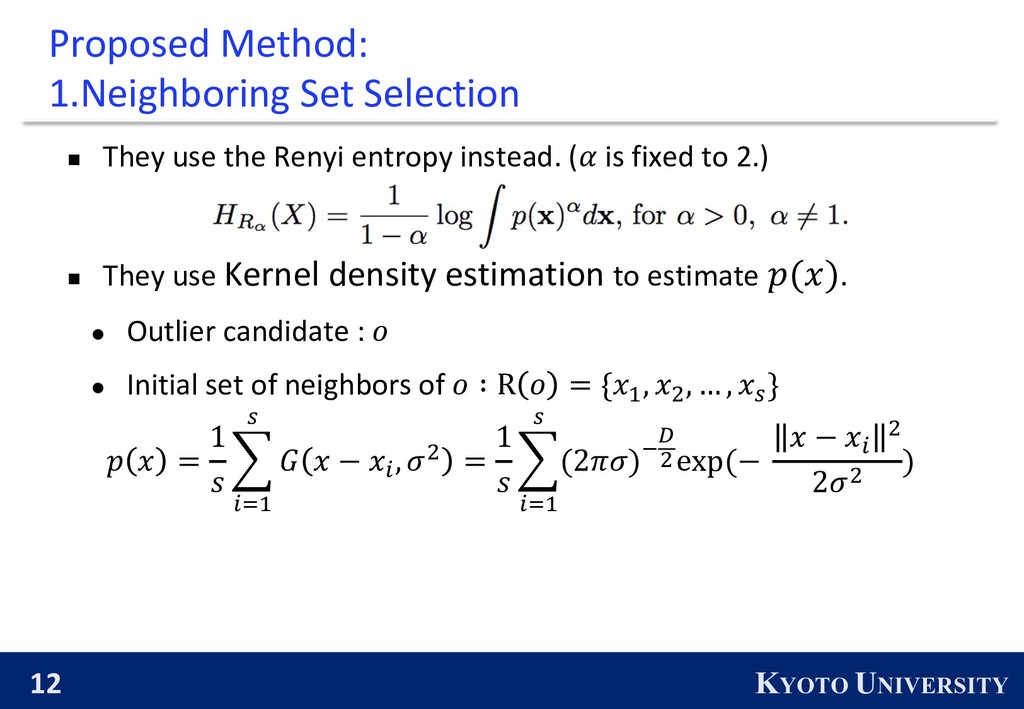
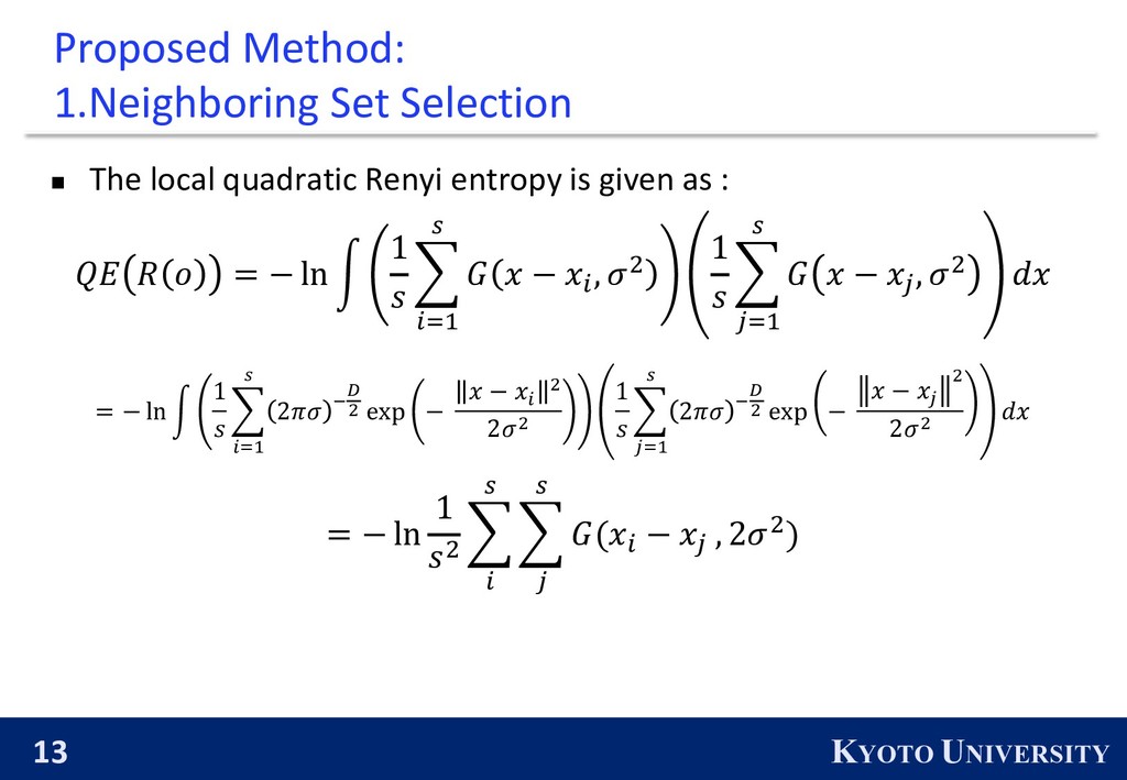
12. 12 KYOTO UNIVERSITY Proposed Method: 1.Neighboring Set Selection n They use the Renyi entropy instead. (! is fixed to 2.) n They use Kernel density estimation to estimate "($). l Outlier candidate : & l Initial set of neighbors of & ∶ R & = {$+ , $- , … , $/ } " $ = 1 2 3 45+ / 6 $ − $4 , 8- = 1 2 3 45+ / (2:8); < -exp(− $ − $4 - 28- )
13. 13 KYOTO UNIVERSITY Proposed Method: 1.Neighboring Set Selection n The local quadratic Renyi entropy is given as : !" # $ = − ln ) 1 + , -./ 0 1 2 − 2- , 45 1 + , 6./ 0 1 2 − 26 , 45 72 = − ln ) 1 + , -./ 0 294 : ; 5 exp − 2 − 2- 5 245 1 + , 6./ 0 294 : ; 5 exp − 2 − 26 5 245 72 = − ln 1 +5 , - 0 , 6 0 1(2- − 26 , 245)
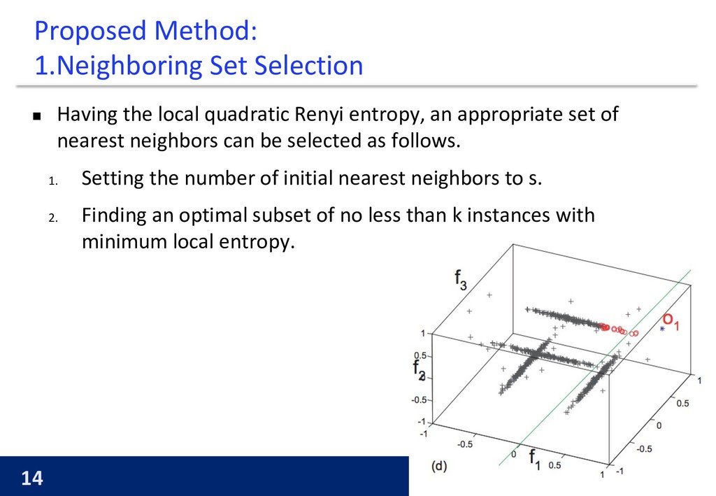
14. 14 KYOTO UNIVERSITY Proposed Method: 1.Neighboring Set Selection n Having the local quadratic Renyi entropy, an appropriate set of nearest neighbors can be selected as follows. 1. Setting the number of initial nearest neighbors to s. 2. Finding an optimal subset of no less than k instances with minimum local entropy.
15. 15 KYOTO UNIVERSITY Proposed Method: 2.Anomaly Degree Computation n Next, they develop a method to calculate the anomaly degree for each object in the dataset X. n Generally, they exploit an approach of local dimensionality reduction. n Notation: l ! : data point under consideration. ! ∈ ℝ$. l & ! : A set of neighboring inliers l ' = [*+ , *- , … , */ ] : Matrix form of & 1 . ' ∈ ℝ/×$.
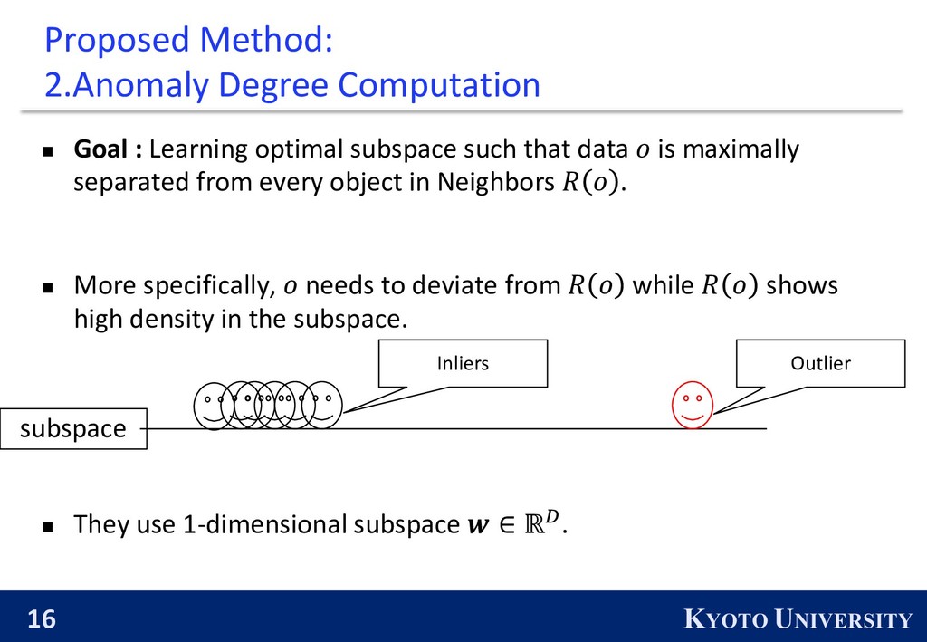
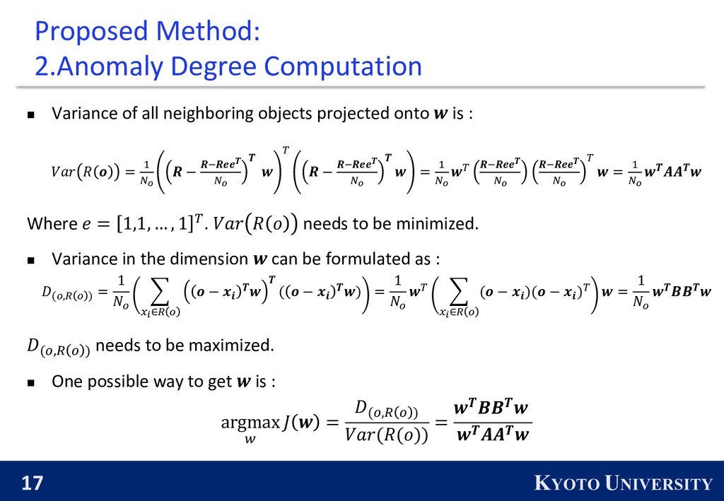
16. 16 KYOTO UNIVERSITY Proposed Method: 2.Anomaly Degree Computation n Goal : Learning optimal subspace such that data ! is maximally separated from every object in Neighbors " ! . n More specifically, ! needs to deviate from " ! while " ! shows high density in the subspace. n They use 1-dimensional subspace # ∈ ℝ&. Outlier Inliers subspace
17. 17 KYOTO UNIVERSITY Proposed Method: 2.Anomaly Degree Computation n Variance of all neighboring objects projected onto ! is : "#$ % & = ( )* + − +-+../ )* / ! 0 + − +-+../ )* / ! = ( )* !0 +-+../ )* +-+../ )* 0 ! = ( )* !/11/! Where 2 = 1,1, … , 1 0. "#$ % 6 needs to be minimized. n Variance in the dimension ! can be formulated as : 7(9,: 9 ) = 1 <9 = >?∈: 9 & − AB /! / ( & − AB /!) = 1 <9 !0 = >?∈: 9 (& − AB)(& − AB)0 ! = 1 <9 !/CC/! 7(9,: 9 ) needs to be maximized. n One possible way to get ! is : argmax I J ! = 7(9,: 9 ) "#$(%(6)) = !/CC/! !/11/!
18. 18 KYOTO UNIVERSITY Proposed Method: 2.Anomaly Degree Computation ! !" # $ = ! !" $&''&$ $&((&$ = ''& + (''&)& $ $&((&$ − $&''&$ ((& + (((&)& $ ($&((&$)- n Setting . ./ # $ to 0 results in : 2''&$ $&((&$ = 2$&''&$((&$ ($&((&$)''&$ = ($&''&$)((&$ ''&$ = $&''&$ $&((&$ ((&$ ''&$ = # $ ((&$ (((&)12''&$ = # $ $
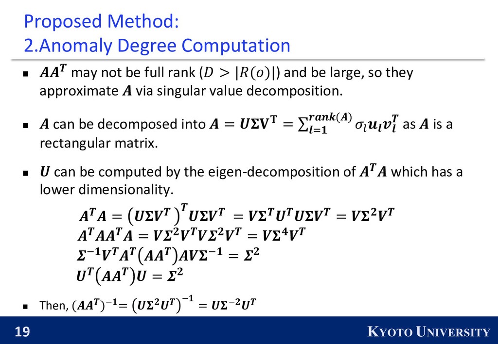
19. 19 KYOTO UNIVERSITY Proposed Method: 2.Anomaly Degree Computation n !!" may not be full rank (# > |&(()|) and be large, so they approximate ! via singular value decomposition. n ! can be decomposed into ! = +,-. = ∑ 012 3456(!) 78 90 :0 " as ! is a rectangular matrix. n + can be computed by the eigen-decomposition of !"! which has a lower dimensionality. !"! = +,;" " +,;" = ;,"+"+,;" = ;,<;" !"!!"! = ;=<;";=<;" = ;,>;" =?2;"!" !!" !;,?2 = =< +" !!" + = =< n Then, (!!")?2= +,<+" ?2 = +,?<+"
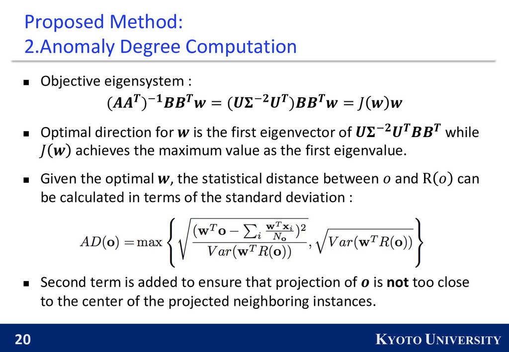
20. 20 KYOTO UNIVERSITY Proposed Method: 2.Anomaly Degree Computation n Objective eigensystem : (""#)%&''#( = (*+%,*#)''#( = - ( ( n Optimal direction for ( is the first eigenvector of *+%,*#''# while - ( achieves the maximum value as the first eigenvalue. n Given the optimal (, the statistical distance between . and R . can be calculated in terms of the standard deviation : n Second term is added to ensure that projection of 0 is not too close to the center of the projected neighboring instances.
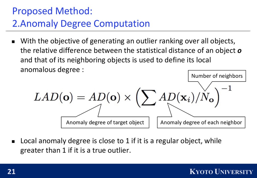
21. 21 KYOTO UNIVERSITY Proposed Method: 2.Anomaly Degree Computation n With the objective of generating an outlier ranking over all objects, the relative difference between the statistical distance of an object o and that of its neighboring objects is used to define its local anomalous degree : n Local anomaly degree is close to 1 if it is a regular object, while greater than 1 if it is a true outlier. Number of neighbors Anomaly degree of each neighbor Anomaly degree of target object
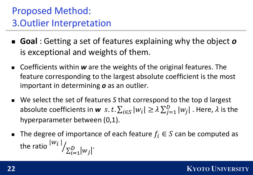
22. 22 KYOTO UNIVERSITY Proposed Method: 3.Outlier Interpretation n Goal : Getting a set of features explaining why the object o is exceptional and weights of them. n Coefficients within w are the weights of the original features. The feature corresponding to the largest absolute coefficient is the most important in determining o as an outlier. n We select the set of features S that correspond to the top d largest absolute coefficients in w !. #. ∑ %∈' |)% | ≥ + ∑ ,-. / |), | . Here, + is the hyperparameter between (0,1). n The degree of importance of each feature 0% ∈ 1 can be computed as the ratio 2 |34 | ∑456 7 38 .
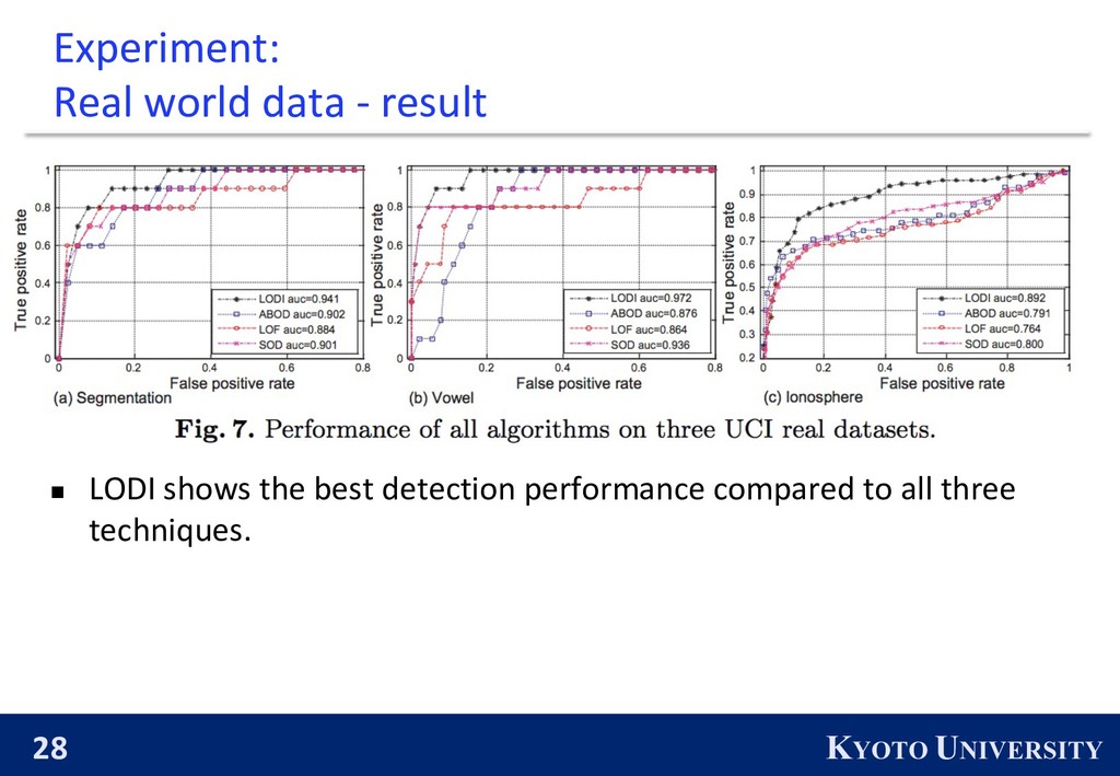
23. 23 KYOTO UNIVERSITY Experiment: Experimental set up n Baselines : l Local Outlier Factor (density-based technique) l ABOD (angle based technique) l SOD (axis-parallel subspace) n They use k=20 as lower bound for the number of kNNs in LODI.
24. 24 KYOTO UNIVERSITY Experiment: Synthetic Data n Synthetic data1, Synthetic data2 and Synthetic data3 l each consists of 50K data instances generated from 10 normal distributions. l For each dimension i-th of a normal distribution, !" is randomly selected from {10, 20, 30, 40, 50} and #" is selected from {10, 100}. Ø Syn1 : percentage of distributions having large variance is 40% Ø Syn2 : percentage of distributions having large variance is 60% Ø Syn3 : percentage of distributions having large variance is 80% l For each dataset, they vary 1%, 2%, 5% and 10% of the whole data as the number of randomly generated outliers and also vary the dimensionality of each dataset in 15,30, and 50.
25. 25 KYOTO UNIVERSITY Experiment: Synthetic Data : comparison of outlier detection rates n LODIw/o : not using the entropy-based approach in kNNs selection n LODI shows the best performance.
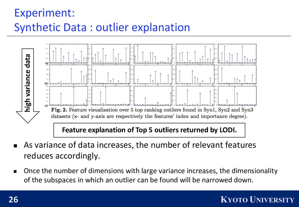
26. 26 KYOTO UNIVERSITY Experiment: Synthetic Data : outlier explanation n As variance of data increases, the number of relevant features reduces accordingly. n Once the number of dimensions with large variance increases, the dimensionality of the subspaces in which an outlier can be found will be narrowed down. high variance data Feature explanation of Top 5 outliers returned by LODI.
27. 27 KYOTO UNIVERSITY Experiment: Real world data 1. Image segmentation data : 16 attributes 2. Vowel data : 10 attributes 3. Ionosphere data : 32 features n They downsample several classes and treat them as outliers.
28. 28 KYOTO UNIVERSITY Experiment: Real world data - result n LODI shows the best detection performance compared to all three techniques.
29. 29 KYOTO UNIVERSITY Experiment: Real world Data : outlier explanation Feature explanation of Top 5 outliers returned by LODI.
30. 30 KYOTO UNIVERSITY Conclusion and Challenges: n They develop the LODI algorithm to address outlier detection and explanation at the same time. n Experiments on both synthetic and real-world datasets demonstrated the appealing performance of LODI and its interpretation form over outliers is intuitive and meaningful. n limitation of LODI : 1. Computation is expensive. 2. LODI assumes that an outlier can be linearly separated from inliers. Ø Nonlinear dimensionality reduction can be applied. Ø But how can we interpret nonlinear outliers?