SAVE: A large scale randomised control trial approach to testing domestic electricity consumption flexibility in the UK

Otago Energy Research Centre Seminar, March 1st 2018

Abstract:

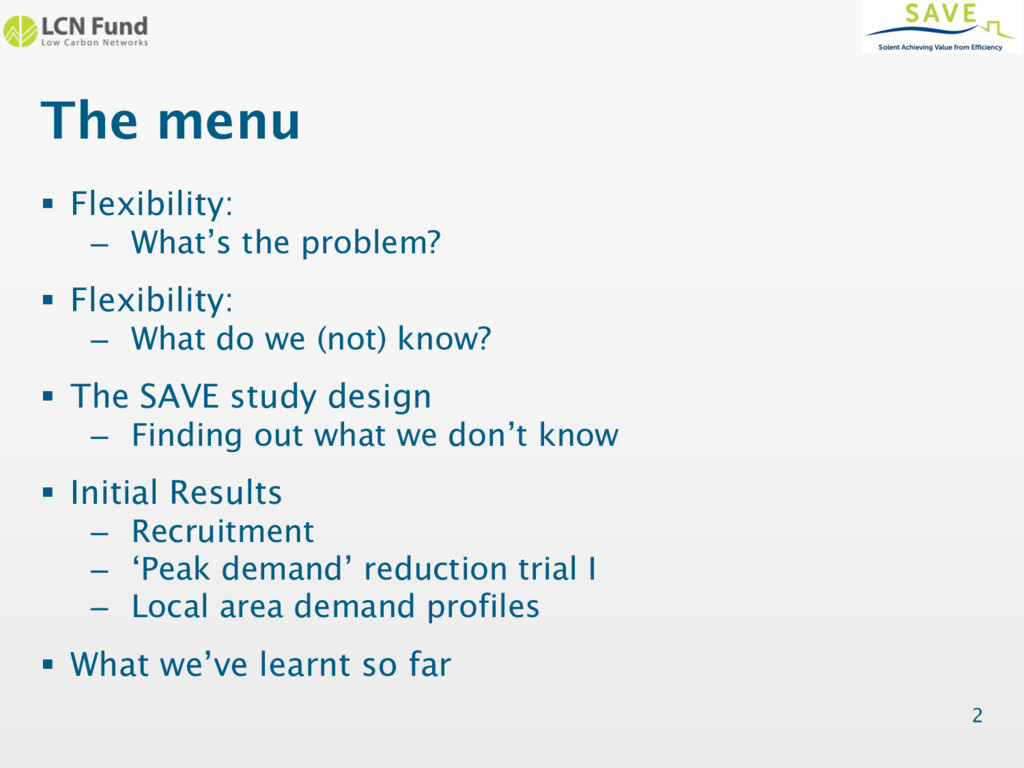
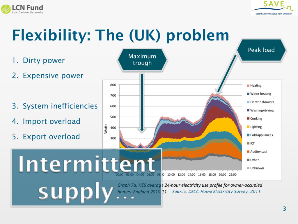
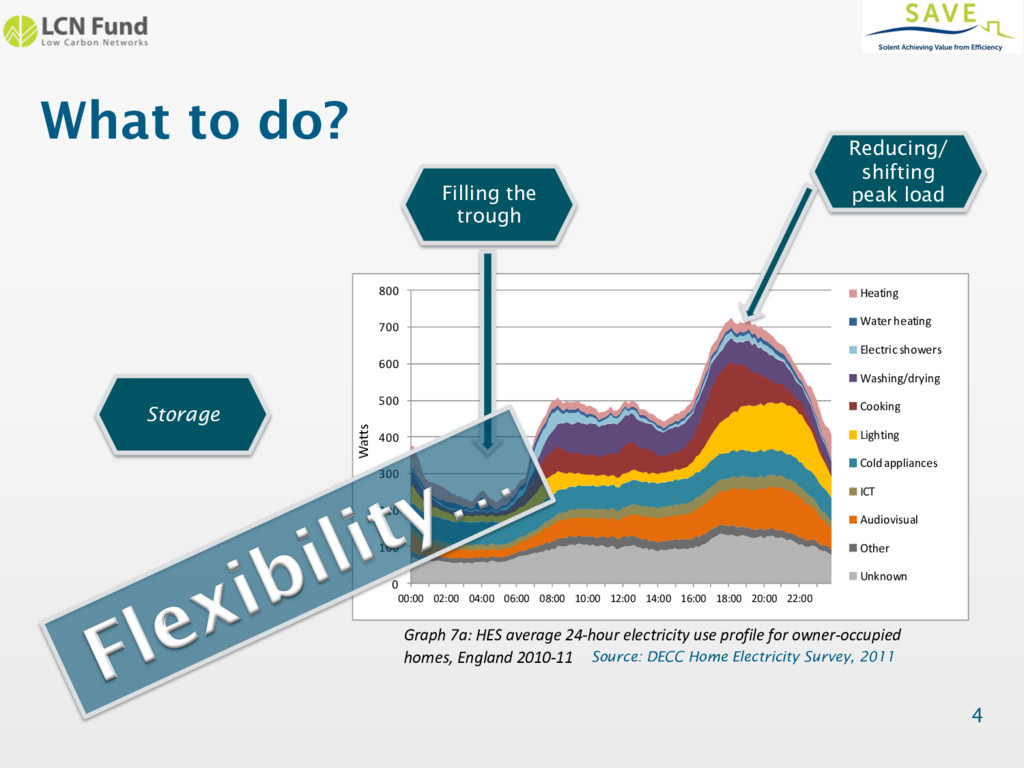
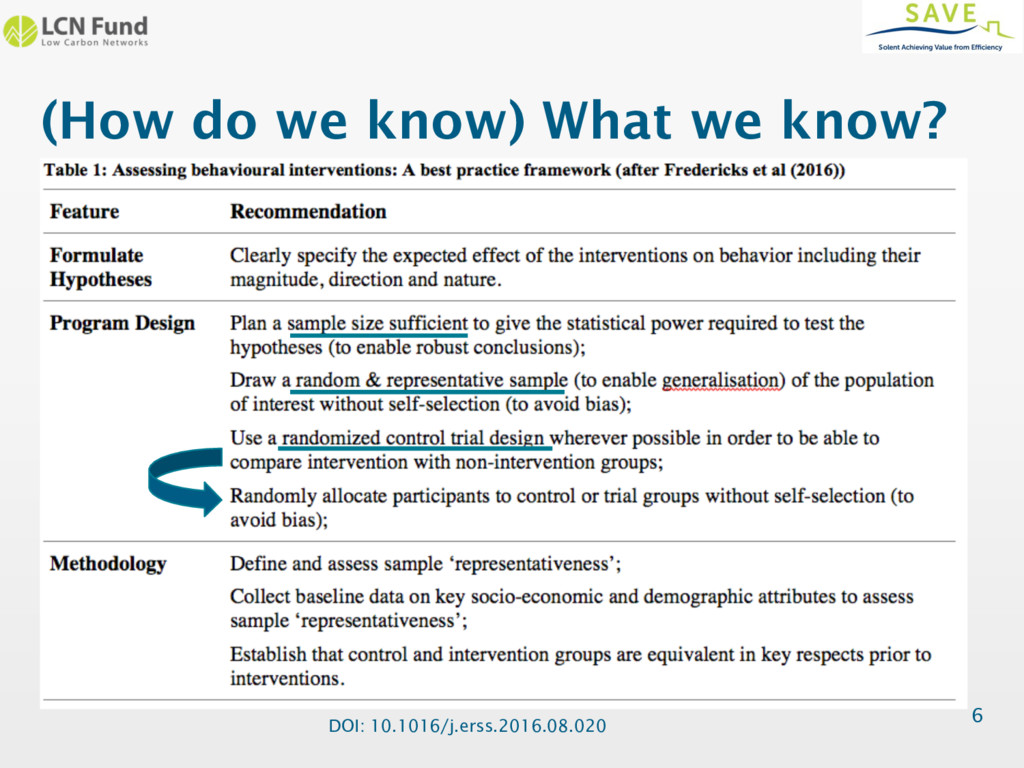
“Whilst overall reduction of energy demand is receiving increasing policy attention in the United Kingdom, reductions targeted at specific times of day are also becoming crucial. This is largely driven by the need to reduce the effects of regular evening demand peaks of increasing magnitude on an ageing local distribution infrastructure; to reduce reliance on ‘high-carbon high-cost’ fuel sources during such demand peaks and to attempt to better match demand to localised, time-specific or intermittent low-carbon generation. This presentation will describe SAVE, a large scale randomised control trial approach to testing a range of interventions intended to reduce and/or shift electricity consumption out of the ‘peak’ 16:00-20:00 evening winter weekday periods. After describing the participant recruitment process and demonstrating the representative and thus generalisable nature of the resulting sample, the presentation will present preliminary results of the first trial period testing different forms of financial and non-financial incentives. It will conclude with a glimpse of ongoing work to use the results to model local area demand profiles which is being continued at the University of Otago in 2018-2019 under an EU funded Marie Skłodowska-Curie Global Fellowship.”

Transcript

1. SAVE Ben Anderson b.anderson@soton.ac.uk @dataknut Tom Rushby t.w.rushby@soton.ac.uk @tom_rushby A large scale randomised control trial approach to testing domestic electricity consumption flexibility in the UK
2. The menu § Flexibility: – What’s the problem? § Flexibility: – What do we (not) know? § The SAVE study design – Finding out what we don’t know § Initial Results – Recruitment – ‘Peak demand’ reduction trial I – Local area demand profiles § What we’ve learnt so far 2
3. Flexibility: The (UK) problem 3 1. Dirty power 2. Expensive power 3. System inefficiencies 4. Import overload 5. Export overload 3 UK Housing Energy Fact File Graph 7a: HES average 24-hour electricity use profile for owner-occupied homes, England 2010-11 Gas consumption 0 100 200 300 400 500 600 700 800 00:00 02:00 04:00 06:00 08:00 10:00 12:00 14:00 16:00 18:00 20:00 22:00 Heating Water heating Electric showers Washing/drying Cooking Lighting Cold appliances ICT Audiovisual Other Unknown Watts Peak load Source: DECC Home Electricity Survey, 2011 Maximum trough Intermittent supply…
4. What to do? 4 UK Housing Energy Fact File Graph 7a: HES average 24-hour electricity use profile for owner-occupied homes, England 2010-11 Gas consumption 0 100 200 300 400 500 600 700 800 00:00 02:00 04:00 06:00 08:00 10:00 12:00 14:00 16:00 18:00 20:00 22:00 Heating Water heating Electric showers Washing/drying Cooking Lighting Cold appliances ICT Audiovisual Other Unknown Watts Reducing/ shifting peak load Source: DECC Home Electricity Survey, 2011 Filling the trough Storage Flexibility…
5. What do we know? 5
6. (How do we know) What we know? 6 DOI: 10.1016/j.erss.2016.08.020
7. § There have been quite a lot of ‘demand response’ trials § We reviewed over 30 major (published) studies How does the literature stack up? 7 “a representative random sample of households with random allocation to control and intervention groups of sufficient size to robustly detect the effect observed was achieved only by the Irish Smart Meter trial.” @tom_rushby
8. What do we know? 8 “a representative random sample of households with random allocation to control and intervention groups of sufficient size to robustly detect the effect observed was achieved only by the Irish Smart Meter trial.” @tom_rushby Not a lot. Well, OK we do know a few things but they are mostly neither statistically robust nor generalizable
9. The menu § Flexibility: – What’s the problem? § Flexibility: – What do we (not) know? § The SAVE study design – Finding out what we don’t know § Initial Results – Recruitment – ‘Peak demand’ reduction trial I – Local area demand profiles § What we’ve learnt so far 10
10. SAVE Objectives § Test ‘Demand Response’ interventions: 11 Households 1. Data informed engagement Other trials suggest reductions of around 6% 2. Data informed engagement + price signals Other trials suggest reductions of around 6- 7% 3. LED lighting trials Lighting is responsible for 19% of evening peak demand
11. SAVE Design Criteria 12 • => Random sample • => Large enough sample Statistically robust: •=> Representative sample Generalisable: •=> Randomly allocated trial & control groups Controlled Image source: pixabay.com
12. Large ‘enough’? 13 0 2 4 6 8 10 12 14 200 400 600 800 1000 1200 1400 Detectable % effect (p = 0.05) Trial Group Size Required Designed effect size Required trial group size Source: UoS analysis of Irish CER Domestic Demand Response pre-trial consumption data Mean kWh 16:00 – 20:00 (“Evening peak”) p = 0.05, P = 0.8 Statistical Pow er Analysis => Each trial group > 1000
13. Recruitment process •Hampshire, Isle of Wight, Southampton, Portsmouth Select study area •Stratify census areas by deprivation quintile •Randomly select n census areas within deprivation quintiles •Randomly select 50 address per census area from PAF Select Addresses •Letter sent by research agency Contact •Field visit: research agency staff Survey & install kit 14 4,318 households 32,000 letters
14. SAVE: Study Design Trial Period 3 Trial Period 2 Trial Period 1 Trial Groups Survey Representative Random Sample N > 4000 Group 1: Control Group 2: (LEDs) Group 3: (Engagement) Group 4: (Engagement + £) 15 Update surveys & Time Use Diaries Update surveys & Time Use Diaries Update surveys & Time Use Diaries Random allocation
15. What was done first § Install Meter Clamp – ‘30 minute’ Wh § 20 minute household survey – Deferred to telephone/web 16 Clamp Database UoS
16. Who remembers this? 17
17. What was done next § Re-install Meter Clamp – 30 15 minute Wh • ~ 414k records/day (130Mb/week) – 10 second W • ~ 37m records/day (11Gb/week) § 20 minute household survey – Deferred to telephone/web – ~ 80% response § Control Group – Yearly update surveys § Trial Groups – Yearly update surveys – Interventions 18 Navetas Loop AWS S3 UoS
18. And now…! 19 N observati ons per day (max 96)
19. The menu § Flexibility: – What’s the problem? § Flexibility: – What do we (not) know? § The SAVE study design – Finding out what we don’t know § Initial Results – Recruitment – ‘Peak demand’ reduction trial I – Local area demand profiles § What we’ve learnt so far 20
20. Testing sample bias 21 § Age § Occupancy Error bars: 95% Confidence Intervals Source: UoS analysis of SAVE vs Understanding Society Wave 4 sample for South East England (weighted for non-response)
21. Testing sample bias 22 § Income § Environmental attitudes Error bars: 95% Confidence Intervals Source: UoS analysis of SAVE vs Understanding Society Wave 4 sample for South East England (weighted for non-response)
22. Illustrative results: daily profiles 23 Household Response Person: Employment status Error bars: 95% CI (assuming normality) Sunday Peak?
23. Illustrative results: daily profiles 24 Dwelling: Main heat source Error bars: 95% CI (assuming normality) N = 120 N = 18 N = 155 N = 2,581
24. The menu § Flexibility: – What’s the problem? § Flexibility: – What do we (not) know? § The SAVE study design – Finding out what we don’t know § Initial Results – Recruitment – ‘Peak demand’ reduction trial I – Local area demand profiles § What we’ve learnt so far 25
25. Trial 1 4-8: Preliminary results 26 • Weekly coms ◦ Jan – Feb 2017 • 16:00 – 20:00 period ◦ Control Group • Nothing ◦ Group 2 • Online & postal ◦ Group 3 • Online only ◦ Group 4 • Postal only SRDC 4 Evidence Report SSET206 SAVE Solent Achieving Value from Efficiency Figure 16: Interior page of initial engagement booklet Over the next nine weeks, this booklet was followed up with one general knowledge postcard and five postcards with specific asks, such as: x Waiting until after 8pm to do the washing or running it only with full loads x Waiting until after 8pm to charge mobiles and tablets x Waiting until after 8pm to use the tumble dryer x Waiting until after 8pm to run the dishwasher or using its timer/delay function x Waiting until after 8pm to watch television or turn the television off in rooms that are not being used SRDC 4 Evidence Report SSET206 SAVE Solent Achieving Value from Efficiency Figure 17 Sample Postcard (Front and Back) All three treatment groups received some sort of consumer engagement messaging: x Group 2 received emails and web portal notifications x Group 3 (data informed engagement and price signals) received emails, web portal Basically nothing much happened
26. Trial 1 4-8: Preliminary results 28 SRDC 4 Evidence Report SSET206 SAVE Solent Achieving Value from Efficiency Page 44 The price levels in TP1 were determined based upon analysis put together in the SAVE business case (Appendix N of full submission) and ensuring any level was deemed market competitive (this is important to consider for aggregator models of domestic DSR). Given the ‘event day’ structure of the trials present clear similarities to National Grid’s triads; commercial analysis was performed between average household demand and £/kW payment levels for triads, the outcome of which suggested a £10 incentive would require at least a 7% load-reduction from each household to be cost-competitive. Accounting behavioural economics in this equation it was determined that consumer responsiveness would benefit from a more relatable, less precise figure of load-reduction and hence this was rounded to 10% for £10. Below is an example of the email message group 2 received two days before the event day. Group 3 received a similar email but with a note about the incentive. Figure 18: Event day messaging 5.2 Trial Outcomes 5.2.1 LED Trial As described earlier, mailers directed the LED trial participants to http://saveled.co.uk, which was set up by RS Components. This website allowed participants to purchase discounted LEDs from a • Specific Day ◦ 15th March 2017 • 16:00 – 20:00 period ◦ Control Group • Nothing ◦ Group 2 • Messages ◦ Group 3 • Messages + • £ Incentive A few interesting things happened • Weekly coms ◦ Jan – Feb 2017 • 16:00 – 20:00 period ◦ Control Group • Nothing ◦ Group 2 • Online & postal ◦ Group 3 • Online only ◦ Group 4 • Postal only Basically nothing much happened Source: pixabay.com
27. Trial 1 4-8 Event: Preliminary results Figure 5: Temporal profiles of consumption around the event day (with 95% CI) The set of charts below in Figure 6 show the overall mean for the 16:00 - 20:00 periods of each day compared to the 4 hours before/after and as above, the 95% confidence intervals give an indication of the statistical significance of any numerical difference. Ben Anderson 5/7/2017 14:58 Deleted: 9 Ben Anderson 5/7/2017 14:58 Deleted: Figure 10 29 Day before Day of Day after
28. Figure 6: Mean 15 minute Wh per period during pre/event/post-event day The charts suggest that: • On the day preceding the event day: Group 3 appeared to use more than the other groups during the evening peak period which would be the case if consumption had been shifted to Ben Anderson 5/7/2017 14:58 Deleted: 10 Trial 1 4-8 Event: Preliminary results 30 Day before Day of Day after
29. Trial 1 4-8 Event: Pre-peak models 31 Intervention (n = 2,859) Intervention + email (n = 2,859) Intervention + email + ‘env score’ (n = 2,199) ??
30. Trial 1 4-8 Event: Peak period models 32 Intervention (n = 2,859) Intervention + email (n = 2,859) Intervention + email + ‘env score’ (n = 2,199)
31. Trial 1 4-8 Event: Results summary Pre 4-8 pm • Group 3 (£ incentive): +5% (95% CI : -3% to +15%) • Especially where opened pre-event email (extra +2%) 4-8 pm • Group 2: -3% (-11% to +5%) • Group 3 (£ incentive): -1% (-9% to +7%) • Especially where opened pre-event email (extra -2%) • Possibly correlates with ’going/staying’ out of home After 8 pm • Group 2: +4% (-4% to +12%) • Group 3: +6% (-2% to +15%) 33
32. The menu § Flexibility: – What’s the problem? § Flexibility: – What do we (not) know? § The SAVE study design – Finding out what we don’t know § Initial Results – Recruitment – ‘Peak demand’ reduction trial I – Local area demand profiles § What we’ve learnt so far 34
33. Modeling ‘local’ flexibility § What we know (now): – Sample kWh profiles – Effects of interventions § What we want to know: – Where is the demand? – Who might shift & where are they? 35 1. Targeted interventions 2. Network investment decisions £££
34. Modeling ‘local’ flexibility 36 1. Targeted interventions 2. Network investment decisions £££ Source: maps.google.co.uk
35. Modeling ‘local’ flexibility Synthetic Electricity Census UK Census 2011 SAVE survey & kWh data 37 6,136 Output Areas (c 100 households) Source: http://datashine.org.uk
36. Example results: Baseline 39 To illustrate the output from the small area estimation, two highly contrasting OAs are selected as the ‘target’ areas: x the OA with highest % of single person households: E00167003 x the OA with the lowest % of single person households: E00115898 The OAs have been selected in this way to provide test cases that tease out any limitations in the modelling technique. The household counts for these OAs are shown in Table 20 and the resulting weighted household counts are expected to match these. Table 20 Census counts and % single-person households for selected OAs OA Code Total household count Number of single- person households % single-person households E00115898 85 0 0 E00167003 200 182 91 The OA with the lowest percentage of single-person households (0 households, 0%) has 85 households in total, whilst the OA with the highest percentage (182 households, 91%) has rather more at 200. As each of the four illustrative models described in Section 5.1 above will draw upon the consumption data from a different pool of SAVE sample households, the weighting file generated by the IPF procedure for each separate model is applied to each of the two OAs in turn. The following sections describe briefly the results gained from each model. The results for each model include tables to illustrate that each of the different treatment groups produce different ‘pools’ of SAVE households, and that the weights resulting from the IPF process change according to their different characteristics. 5.6.1 Baseline model (all households) Having established that two quite different OAs have been selected, kWh profile data for the first (non-holiday) Sunday in January 2017 (8/1/2017) is attached as a ‘baseline’ test. Half-hourly (sum) kWh consumption data is merged to the households that were pushed through the IPF process.19 First, the weighted counts for each household size type (single, two person etc) are checked. Table 21 contains the number of households in the SAVE sample ‘pool’ (N unweighted column) for each household size in both test OAs, along with the mean, minimum and maximum weights that the IPF Source: http://datashine.org.uk SAVE-SDRC-2.2-Updated-Customer-Model-v2.3_final.docx PROJECT CONFIDENTIAL Figure 24 Simulated OA consumption profiles by household size (colours indicate number of people in household), baseline data, all groups The analysis is repeated for the mean kWh for households by size (Figure Sunday 8th January 2017 ??
37. The menu § Flexibility: – What’s the problem? § Flexibility: – What do we (not) know? § The SAVE study design – Finding out what we don’t know § Initial Results – Recruitment – ‘Peak demand’ reduction trial I – Local area demand profiles § What we’ve learnt so far 41
38. What have we learnt (so far)? Do: Mind the gaps Record provenance Practice on samples Use commodity hardware Don’t: Suppress variation Impute or delete Use commodity hardware 42 Patchy GSM #Iridis4 People unplug stuff
39. Questions? § @dataknut § www.energy.soton.ac.uk/tag/save/ § www.energy.soton.ac.uk/tag/spatialec – 2 year EU Global Fellowship @Otago CfS – NZ mesh block demand profile model 43 pixabay.com Watch this space