Geography and Planning University of Liverpool 24th GIS Research UK Conference OS Data Challenge Workshop: London, March 2016 Alexandros (Alekos) Alexiou - Alexandros Alexiou, Alex Singleton, Dani Arribas- bel, Michalis Pavlis, Les Dolega, Alec Davies, Ellen Talbot, Konstantinos Daras, Hai Nguyen and Mark Green
OF ENVIRONMENTAL SCIENCES 1. Introduction There is an increasing interest in spatial data sources that could help improve decision making in a variety of fields, such as public policy and environmental sustainability. Recent technological advancements in the fields of remote sensing and G.I.S. have advanced the volume, quality and speed of data availability. The analysis of this vast reservoir of information can offer new insights in planning, city management and smart cities initiatives (RIBA and ARUP , Designing with data: shaping our future cities, 2013). Defining the nature of neighbourhoods, whether it is retail, industrial or purely residential, can inform stakeholders about the environmental strategies, technology infrastructure and management schemes necessary at the small-area level, enhancing policy effectiveness and reducing application costs.
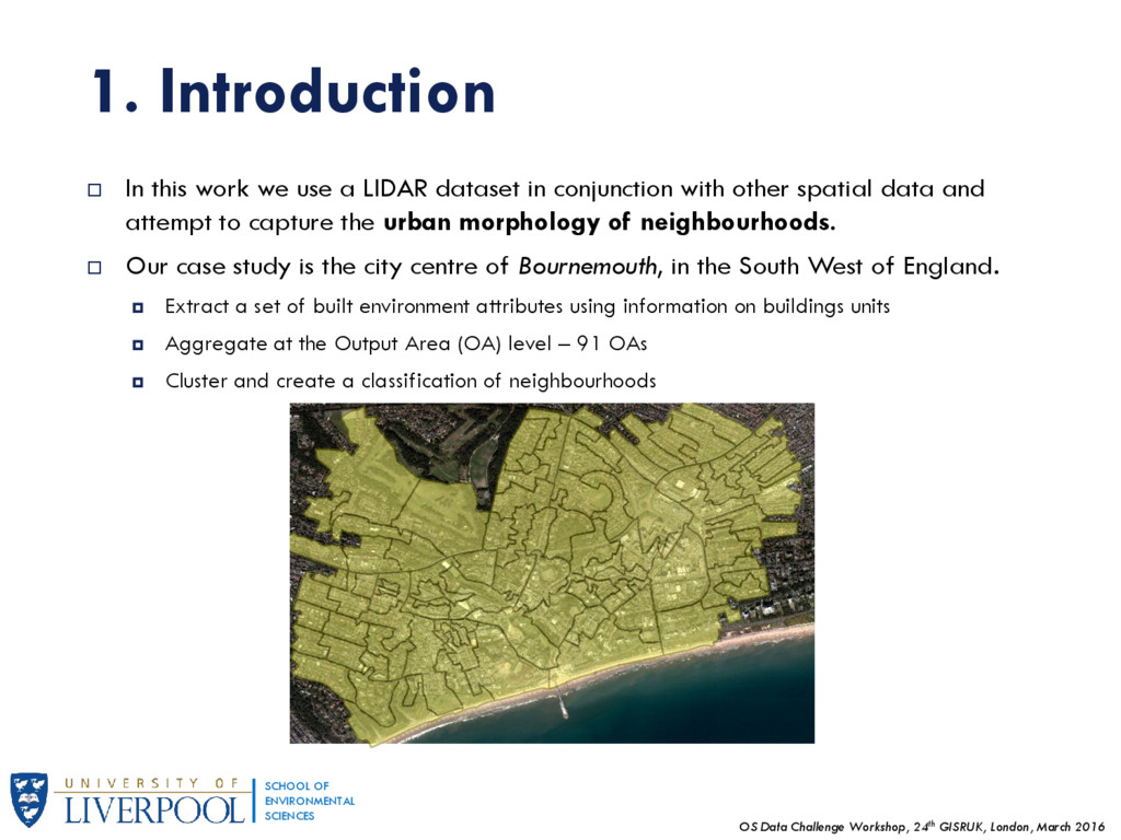
OF ENVIRONMENTAL SCIENCES 1. Introduction In this work we use a LIDAR dataset in conjunction with other spatial data and attempt to capture the urban morphology of neighbourhoods. Our case study is the city centre of Bournemouth, in the South West of England. Extract a set of built environment attributes using information on buildings units Aggregate at the Output Area (OA) level – 91 OAs Cluster and create a classification of neighbourhoods
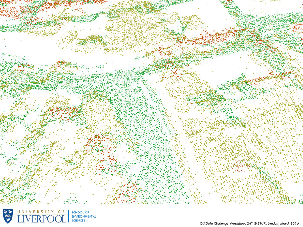
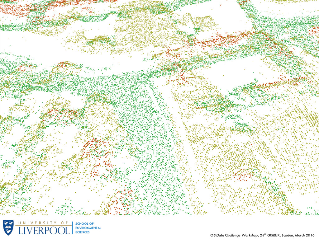
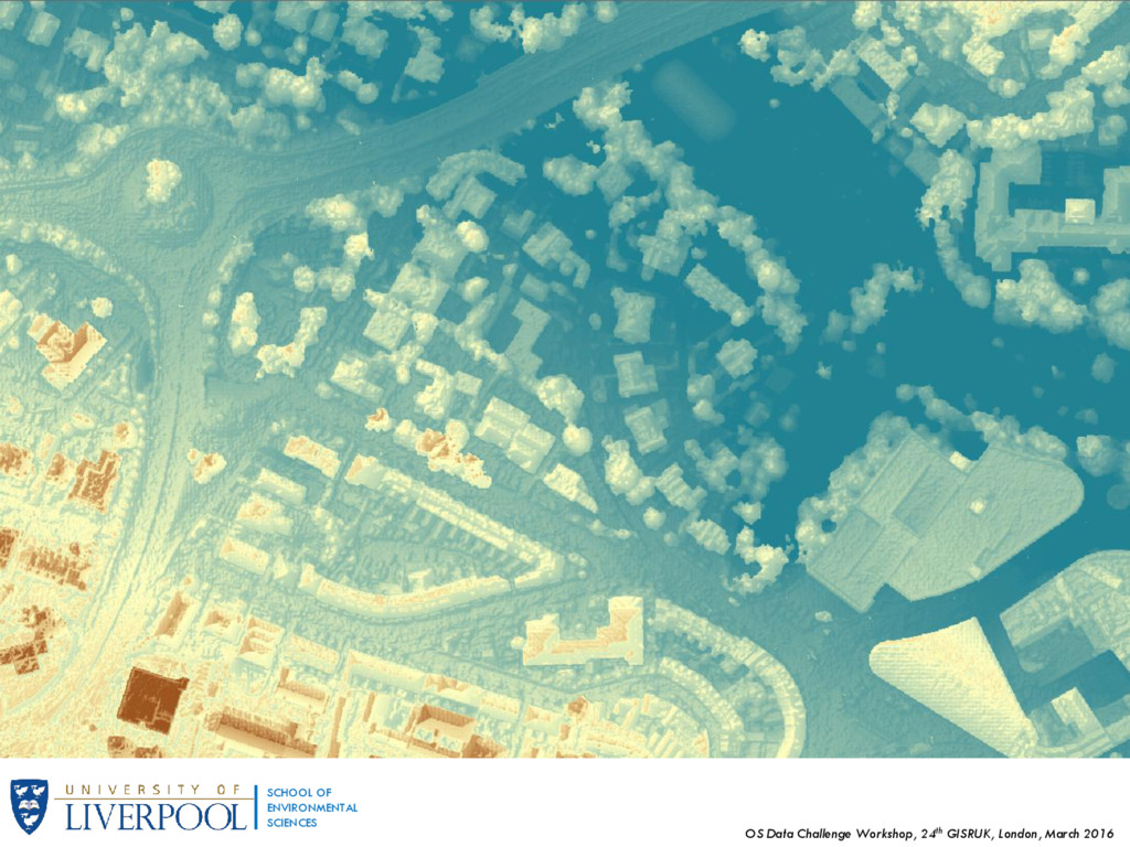
OF ENVIRONMENTAL SCIENCES 2. Methodology and Data Our research area consists of an area roughly covering 815he of the city centre of Bournemouth. Attributes were calculated with on a series of raster calculations and spatial queries using a combination of ArcGIS and R. Datasets Used: 1. LIDAR (Light Detection And Ranging) point data Over 32 million points with, x, y and z coordinates (z being elevation), no information on returns. Average distance between points of 0.499m Converted to a raster Digital Surface Model (DSM) with a cell grid size of 0.5x05m 2. OS Terrain 5 dataset Elevation model with 5m contour line 3. OS Mastermap backdrop Vector data with a variety of features, particularly building polygons 4. Imagery of research area (aerial photograph) 5. OS Maps – Local 6. Retail venues, provided by the ESRC CDRC Point shapefile with 3-tier classification of retail types attached
OF ENVIRONMENTAL SCIENCES 2.1 Buildings A key measure to estimate is the building height: Approximate building volume and density To obtain the building height we subtract the DSM (Digital Surface Model) from a DTM (Digital Terrain Model), so only features above ground level will be measured. DTM data accuracy of 5m was not enough to make accurate estimations; We created a new DTM model using a supervised sample of points across the research area.
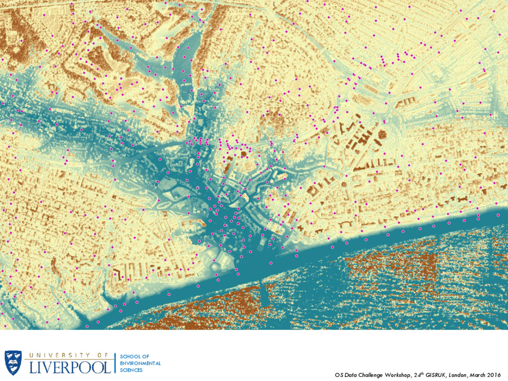
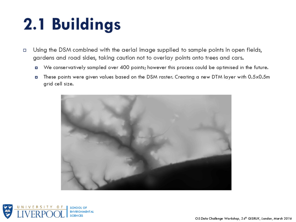
OF ENVIRONMENTAL SCIENCES 2.1 Buildings Using the DSM combined with the aerial image supplied to sample points in open fields, gardens and road sides, taking caution not to overlay points onto trees and cars. We conservatively sampled over 400 points; however this process could be optimised in the future. These points were given values based on the DSM raster. Creating a new DTM layer with 0.5x0.5m grid cell size.
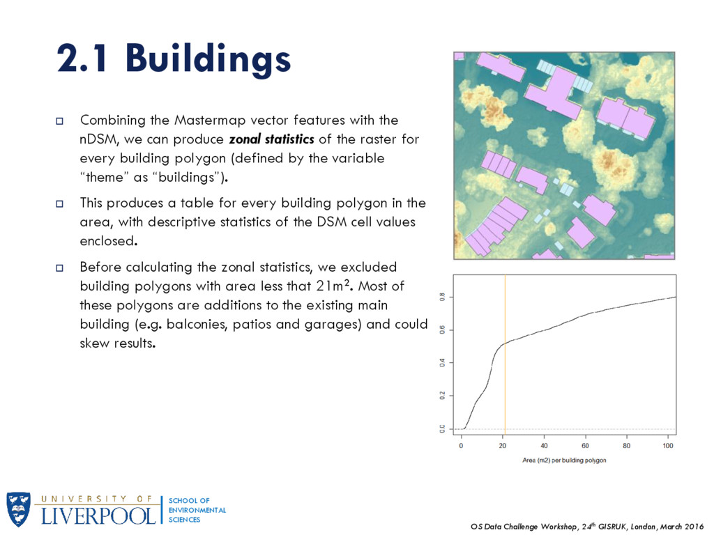
OF ENVIRONMENTAL SCIENCES 2.1 Buildings Combining the Mastermap vector features with the nDSM, we can produce zonal statistics of the raster for every building polygon (defined by the variable “theme” as “buildings”). This produces a table for every building polygon in the area, with descriptive statistics of the DSM cell values enclosed. Before calculating the zonal statistics, we excluded building polygons with area less that 21m2. Most of these polygons are additions to the existing main building (e.g. balconies, patios and garages) and could skew results.
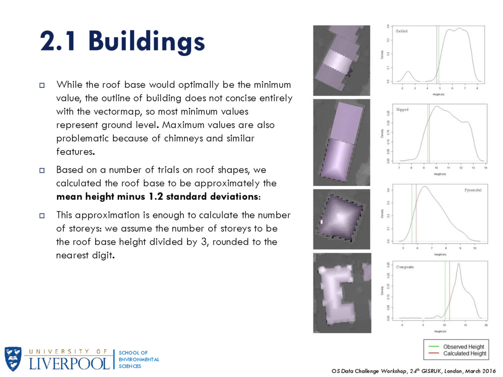
OF ENVIRONMENTAL SCIENCES 2.1 Buildings While the roof base would optimally be the minimum value, the outline of building does not concise entirely with the vectormap, so most minimum values represent ground level. Maximum values are also problematic because of chimneys and similar features. Based on a number of trials on roof shapes, we calculated the roof base to be approximately the mean height minus 1.2 standard deviations: This approximation is enough to calculate the number of storeys: we assume the number of storeys to be the roof base height divided by 3, rounded to the nearest digit.
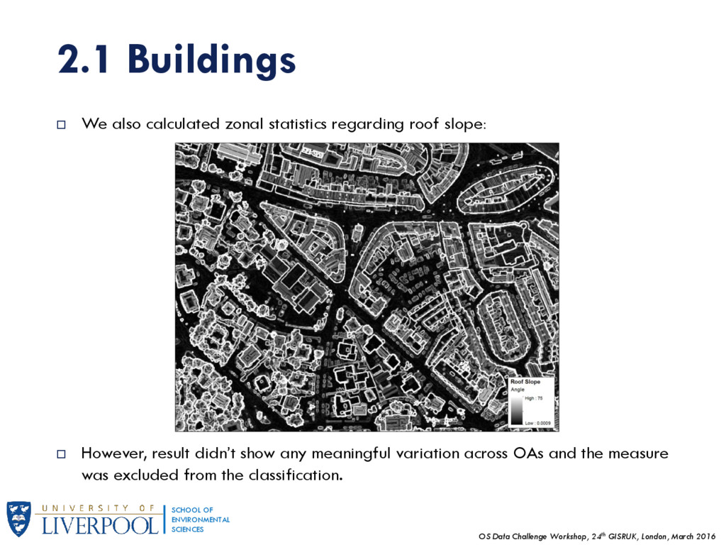
OF ENVIRONMENTAL SCIENCES We also calculated zonal statistics regarding roof slope: However, result didn’t show any meaningful variation across OAs and the measure was excluded from the classification. 2.1 Buildings
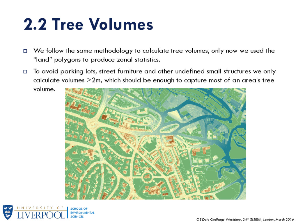
OF ENVIRONMENTAL SCIENCES 2.2 Tree Volumes We follow the same methodology to calculate tree volumes, only now we used the “land” polygons to produce zonal statistics. To avoid parking lots, street furniture and other undefined small structures we only calculate volumes >2m, which should be enough to capture most of an area’s tree volume.
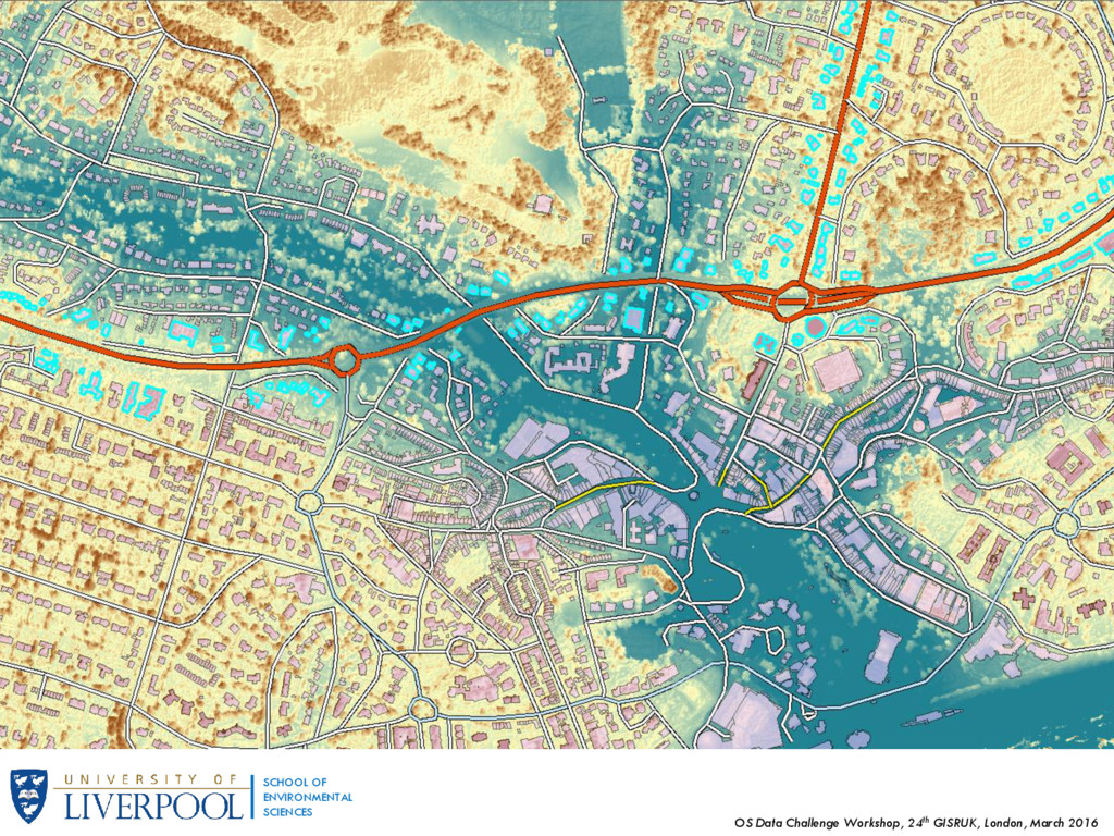
OF ENVIRONMENTAL SCIENCES 2.3 Road Proximity Another attribute that is of importance to land use types is type of road network associated with the area, e.g. crossed by major roads, arterial roads, pedestrian roads, etc. Street network often coincides with OA borders, so simple street-to-area ratios will not suffice. We used proximity-based inputs, which were calculated on a building polygon basis and then attributed to an OA via aggregation. In essence, we performed a series of spatial queries that identified buildings that qualify certain criteria, for instance, “which buildings are within a set distance of a major street?”. The buildings that met each criterion were assigned a corresponding index, weighted by their attributed area and then aggregated per OA. Based on a number of articles regarding proximal effects of built environment characteristics, we conservatively set the proximal distance at 50m. In this instance, we only found useful differentiation for the classes of Major and Pedestrian Roads (as provided by OS Open Map – Local)
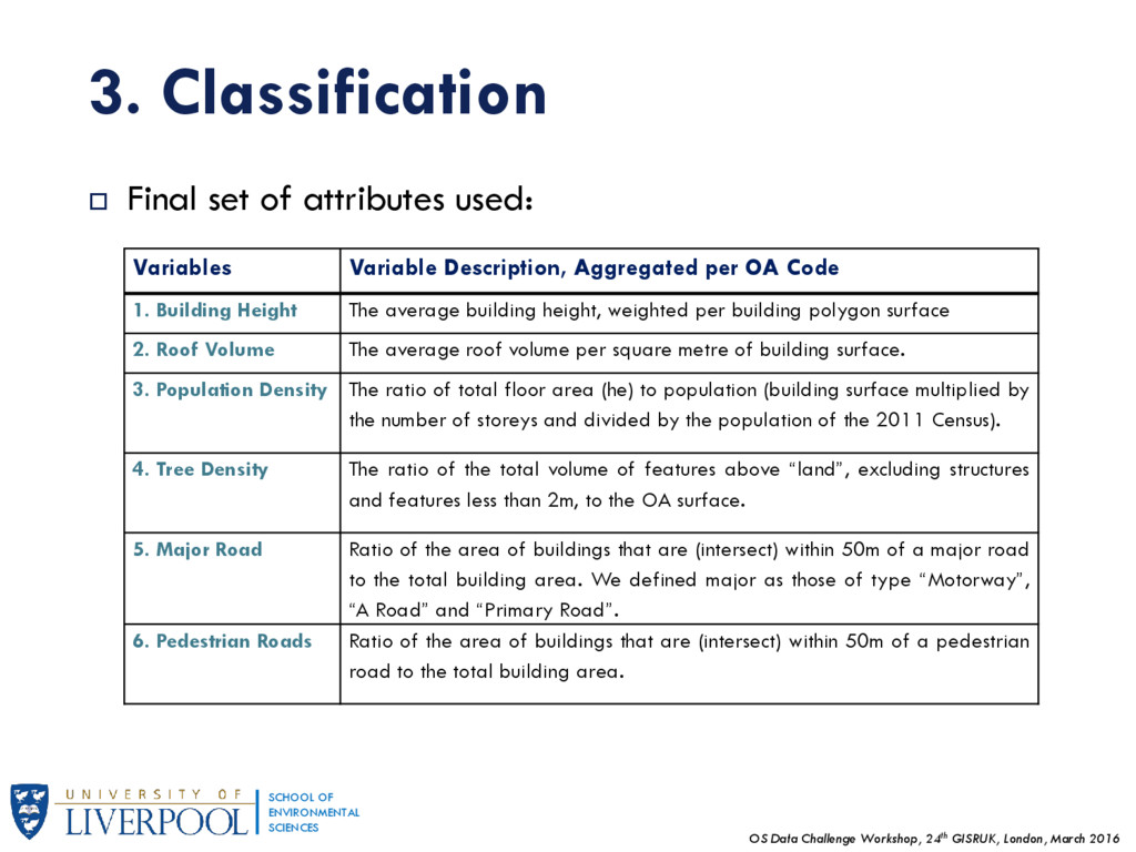
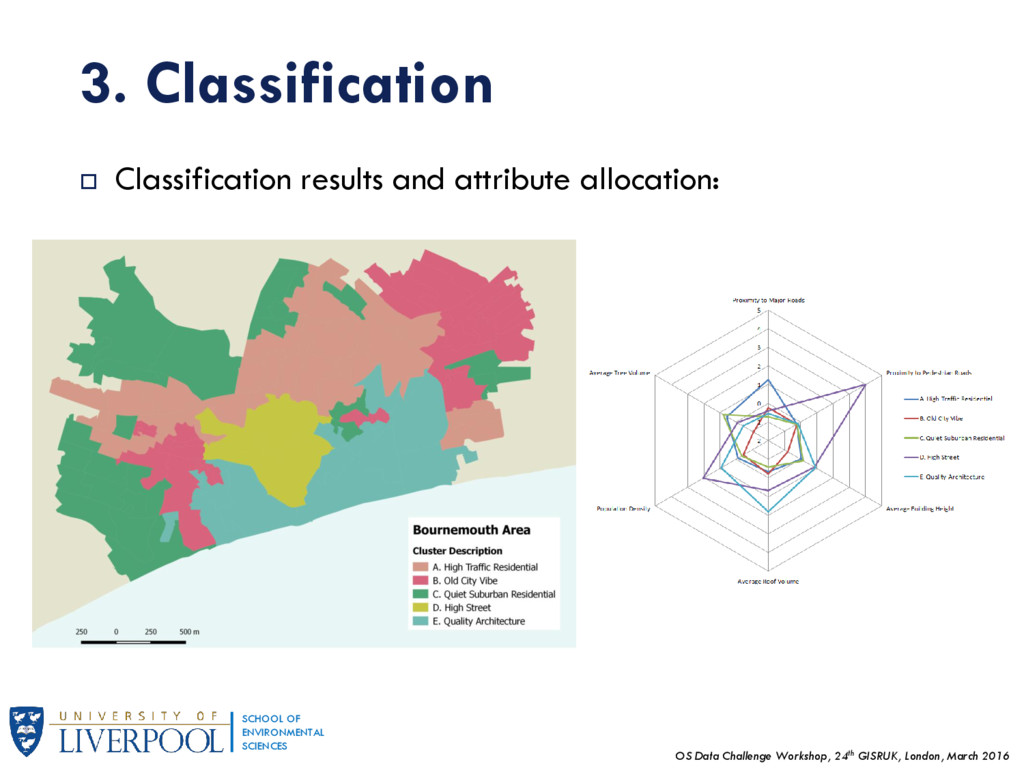
OF ENVIRONMENTAL SCIENCES 3. Classification Final set of attributes used: Variables Variable Description, Aggregated per OA Code 1. Building Height The average building height, weighted per building polygon surface 2. Roof Volume The average roof volume per square metre of building surface. 3. Population Density The ratio of total floor area (he) to population (building surface multiplied by the number of storeys and divided by the population of the 2011 Census). 4. Tree Density The ratio of the total volume of features above “land”, excluding structures and features less than 2m, to the OA surface. 5. Major Road Ratio of the area of buildings that are (intersect) within 50m of a major road to the total building area. We defined major as those of type “Motorway”, “A Road” and “Primary Road”. 6. Pedestrian Roads Ratio of the area of buildings that are (intersect) within 50m of a pedestrian road to the total building area.
OF ENVIRONMENTAL SCIENCES 3. Classification The final dataset includes these six variables across 91 OAs that fall into our research area. Our classification methodology follows a conventional approach, similar to those of socio-economic data in geodemographic analyses, however, comprises only built environment data to create the typology. We used the iterative allocation – reallocation algorithm (K-means) as the clustering technique. We applied a square root transformation and standardized values (z-scores) before the clustering process. Our classification works best for k=5 clusters, since the number of OAs is too small; larger k resulted in very small additional clusters.
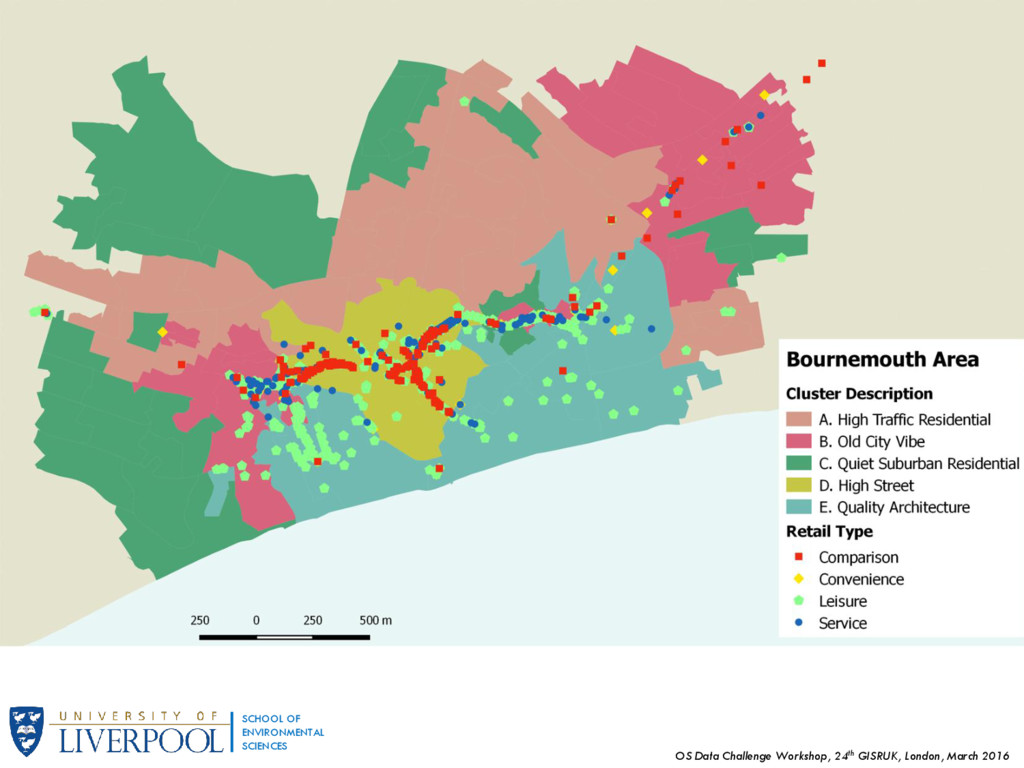
OF ENVIRONMENTAL SCIENCES 3. Classification We can also test the validity of our hypothesis by overlaying data from retail venues. Retail data is supplied as points on the roadside, with an inherent classification based on retail type: Convenience, Comparison, Leisure and Service which further breaks down into two more subcategories. These points were spatially joined to the closest building polygon.
OF ENVIRONMENTAL SCIENCES 3. Classification There are cues in the data that suggest a correspondence of clusters to specific retail types. For instance, the majority of Comparison shops are situated within cluster D – High Street. Cluster E – Quality Architecture represents areas with high concentrations of leisure (mainly hotels) while Cluster B – Old City Vibe appears to have a mixture of retail venues, particularly recreation and service.
OF ENVIRONMENTAL SCIENCES 4. Conclusion While this research certainly suggests an underlying relationship between certain built environment characteristics and the nature of neighbourhoods, a wider and more in-depth approach is needed to consolidate results. It would also be helpful to examine how our classification is responding to: Geographically larger and more diverse areas, Areal types that are not present in the research area, e.g. industrial sites, Broader range of built environment attributes, Fine-tuning. Such a classification can easily be correlated with socio-economic variables and other population data, providing a basis for decision making about the environmental sustainability, data collection strategies and management, particularly within smart city applications.
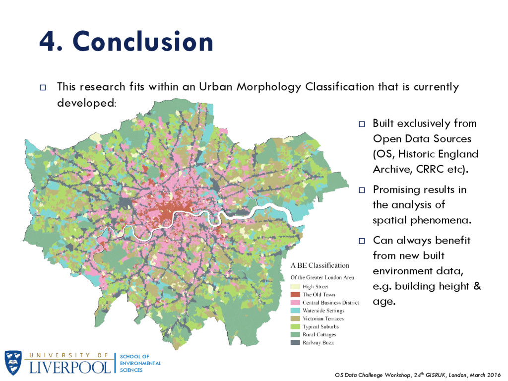
OF ENVIRONMENTAL SCIENCES 4. Conclusion This research fits within an Urban Morphology Classification that is currently developed: Built exclusively from Open Data Sources (OS, Historic England Archive, CRRC etc). Promising results in the analysis of spatial phenomena. Can always benefit from new built environment data, e.g. building height & age.
![Thank you for your time [email protected] http://geographicdatascience.com/team/ https://speakerdeck.com/dblalex](https://files.speakerdeck.com/presentations/5dced756f1594e898bd0c2bd99df9b73/slide_26.jpg)