Geographic Sensitivity: Exploring the Variation of Spatial Autocorrelation Within Geodemographic Classifications

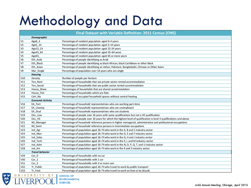
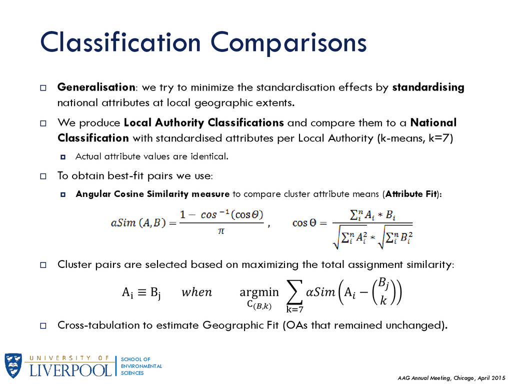
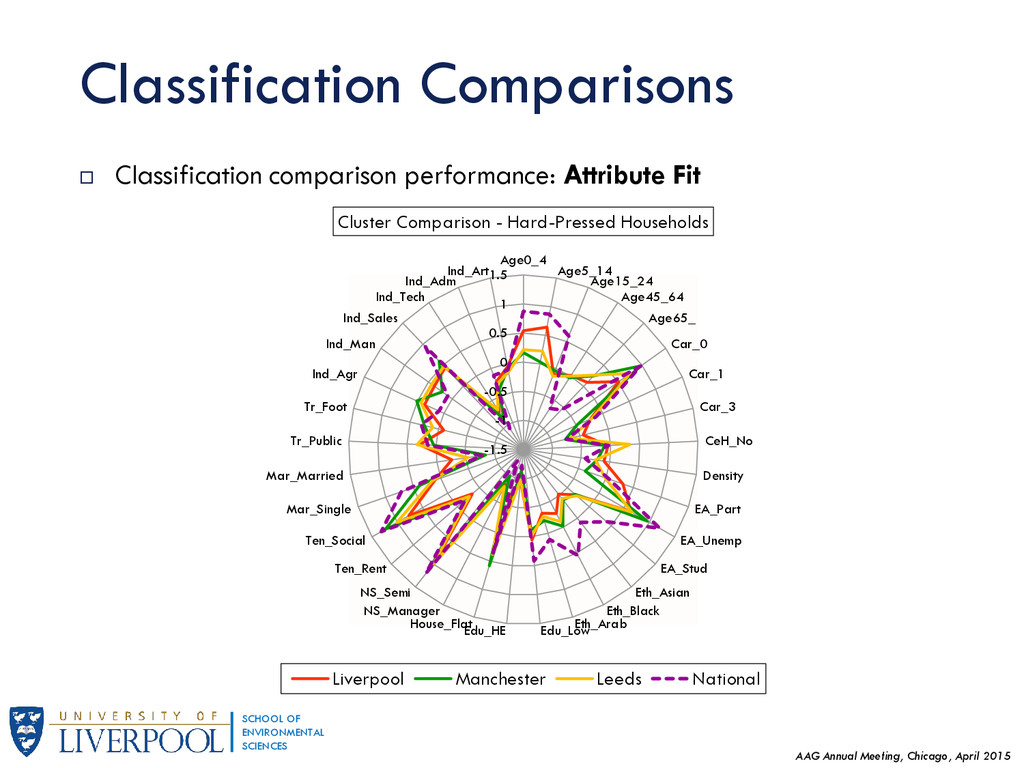
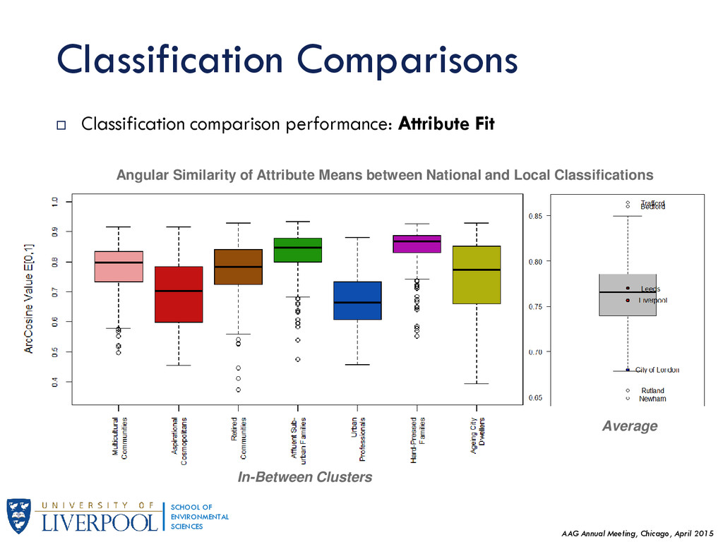
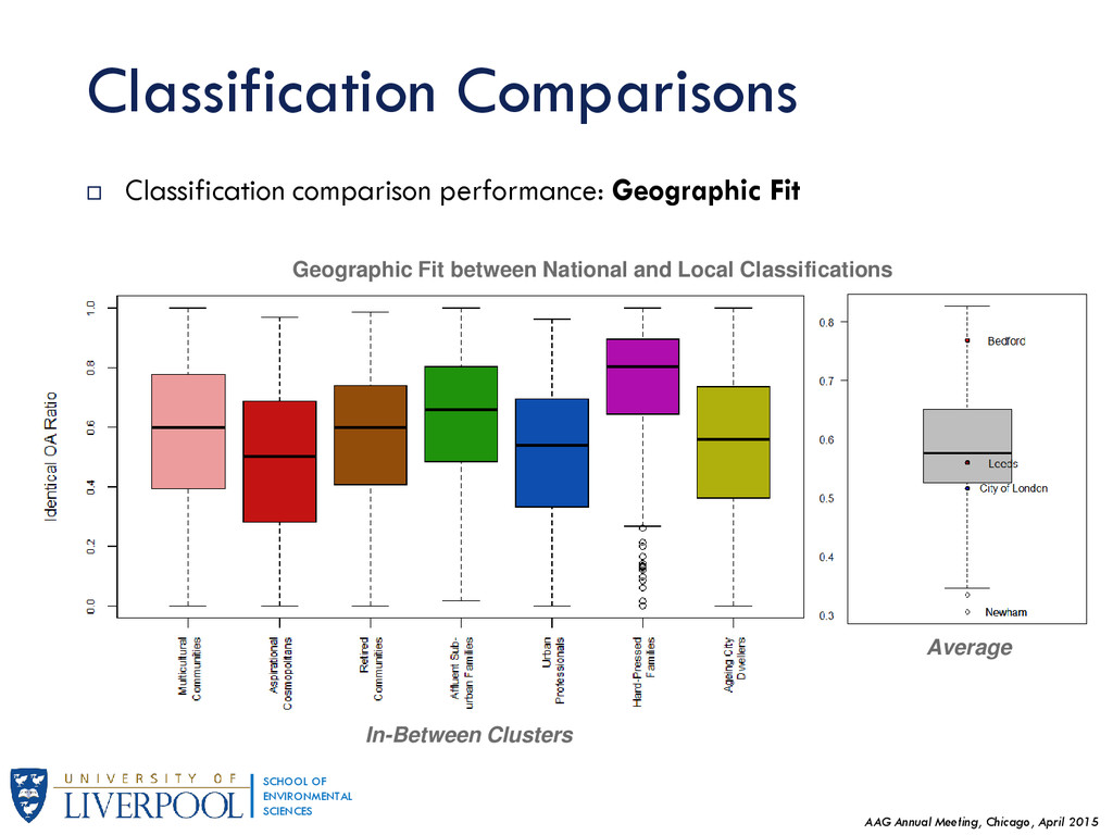
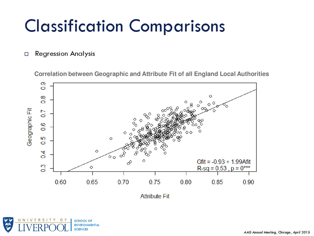
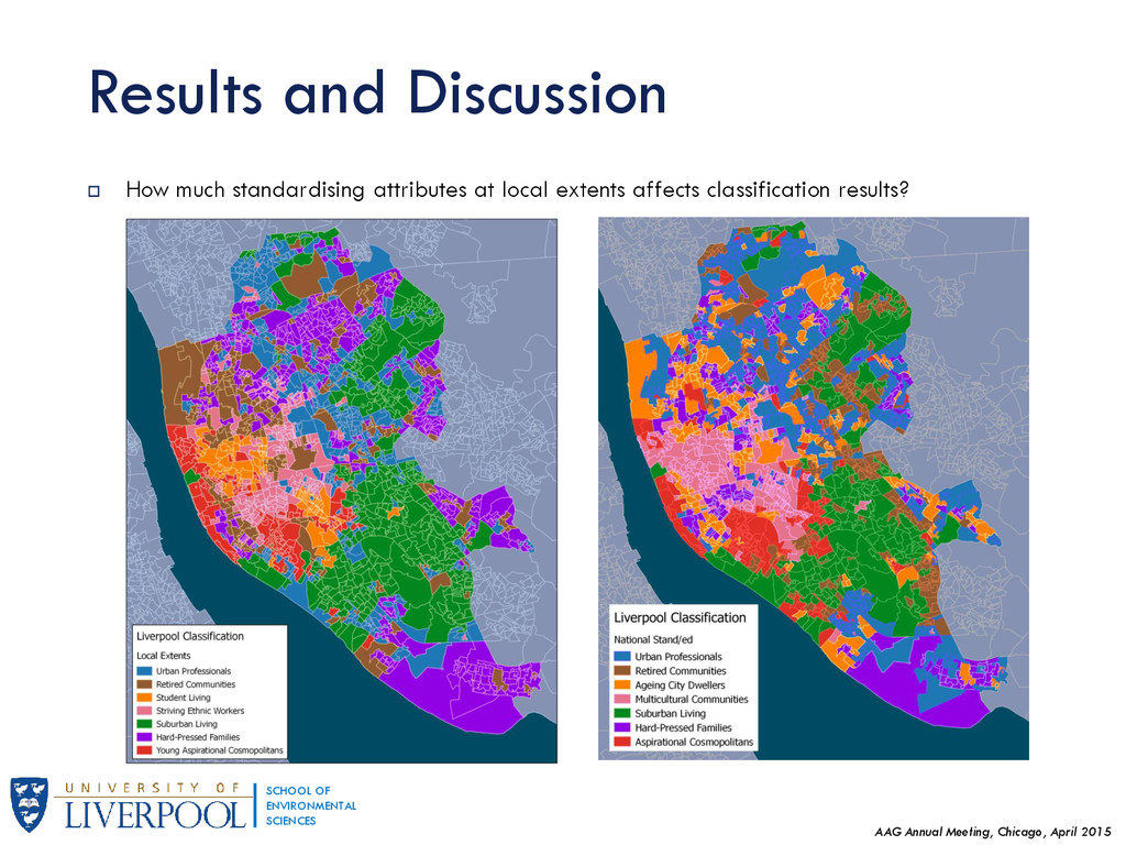
This research generalises results regarding Geographic Sensitivity of socio-spatial patterns (presented earlier in GISRUK 2015) by examining the degree of homogeneity of England's neighbourhoods to national standards. Presented at the Association of American Geographers Annual Meeting in Chicago, April 2015.

Transcript

1. Exploring the Variation of Spatial Autocorrelation Within Geodemographic Classifications AAG Annual Meeting, Chicago, April 2015 Alexandros Alexiou Alex Singleton - Dept. of Geography and Planning University of Liverpool Geographic Sensitivity
2. AAG Annual Meeting, Chicago, April 2015 SCHOOL OF ENVIRONMENTAL SCIENCES Introduction  A Geodemographic Classification (GC) is a data reduction technique that aims to generate through spatial profiling, clusters of populations that share similarities across multiple socio-economic and build environment attributes.  Their composition differs based on the intended stakeholders’ perspective as well as the skills, experience and available data of the creator.  Webber, 1977: pragmatic strategy; what is deemed to work and what is required, alongside some degree of empirical evaluation.  Among the conventional classification systems :  Proprietary classifications primarily designed to describe consumption patterns. Databases are populated not only with census data but compiled from large consumer databases such as credit checking histories, product registrations and private surveys.  MOSAIC (Experian), ACORN (CACI), P2 People and Places (BD), Claritas (PRiZM) and EuroDirect (CAMEO).  Public/Open Classifications: ONS Output Area Classification (OAC) 2001 and 2011.  Similar products have also been created in academia.
3. AAG Annual Meeting, Chicago, April 2015 SCHOOL OF ENVIRONMENTAL SCIENCES Research Outline Main research question:  To what extent do localised classifications deviate from national socio-spatial patterns?  How can this differentiation be measured effectively?  Can a national classification integrate localised patterns? Rationale:  Conventional national classifications may not account for local socio-spatial patterns, increasing the risk of mistargeting when applied locally.  National aggregations sweep away contextual differences between proximal zones.  Researchers without the necessary expertise may find it difficult to produce specific- purpose GCs ad hoc. General-purpose classifications are more convenient to use.  Such debate is long withstanding, originating in the earliest of UK classifications (see Openshaw, Cullingford and Gillard, 1980 and Webber, 1980).
4. AAG Annual Meeting, Chicago, April 2015 SCHOOL OF ENVIRONMENTAL SCIENCES Methodology and Data  This research uses a set of fixed input attributes for Output Area zonal geography to build classifications from different geographic contexts.  For this purpose, administrative areas are considered to demonstrate the impact on final classification outcome when input variables are kept constant.  To illustrate the variation, we look at variations on sets of classifications for Liverpool, and then we proceed to make a model in order to generalise results for all England Local Authorities.  Creation:  Initial 60+ Census 2011 Variables from Demographic, Housing and Economic Activity attributes.  Output Area aggregation level for England (>170.000 neighbourhoods).  K-Means Clustering (Hartigan & Wong, 1979), k=7 single hierarchy (Supergroup Level).  Analysis carried out using the R software.
5. AAG Annual Meeting, Chicago, April 2015 SCHOOL OF ENVIRONMENTAL SCIENCES Methodology and Data  K-Means Input Dataset  Variable formatting:  “Unfit” data: Variable distributions and correlation checks.  Normalisation using Box-Cox Transformation: Obtaining ratios per areal unit Percentages where xa,i is the attribute value i of area a and Pa is the population of reference (denominator) of area a, i.e. total population, number of households, etc. Standardised by group where xa,i is the attribute value i of area a, rN,g is the observed national ratio N for group g and Pa,i is the population of group g in area a. Normalisation Transformation Box – Cox The power λ achieves the best normalization and can be estimated algorithmically. Variable Scaling Z-Score Scaling where xa,i is the attribute value i of area a, μS is the mean and σS is the standard deviation of the set of observations S.  Standardisation (for all geographic scales seperately):
6. AAG Annual Meeting, Chicago, April 2015 SCHOOL OF ENVIRONMENTAL SCIENCES Methodology and Data Final Dataset with Variable Definition: 2011 Census (ONS) Demographic V1 Age0_4 Percentage of resident population aged 0–4 years V2 Age5_14 Percentage of resident population aged 5–14 years V3 Age15_24 Percentage of resident population aged 15-24 years V4 Age45_64 Percentage of resident population aged 45–64 years V5 Age65_ Percentage of resident population aged 65 or more years V6 Eth_Arab Percentage of people identifying as Arab V7 Eth_Black Percentage of people identifying as black African, black Caribbean or other black V8 Eth_Asian Percentage of people identifying as Indian, Pakistani, Bangladeshi, Chinese or Other Asian V9 Mar_Single Percentage of population over 16 years who are single Housing V10 Density Number of people per hectare V11 Ten_Rent Percentage of households that are private sector rented accommodation V12 Ten_Social Percentage of households that are public sector rented accommodation V13 House_Share Percentages of households that are shared accommodation V14 House_Flat Percentage of households which are flats V15 CeH_No Percentage of occupied household spaces without central heating Economic Activity V16 EA_Part Percentage of household representatives who are working part-time V17 EA_Unemp Percentage of household representatives who are unemployed V18 EA_Stud Percentage of household representatives who are students V19 Edu_Low Percentage of people over 16 years with some qualifications but not a HE qualification V20 Edu_HE Percentage of people over 16 years for which the highest level of qualification is level 4 qualifications and above V21 NS_Manager Percentage of household reference persons in higher managerial, administrative and professional occupations V22 NS_Semi Percentage of household reference persons in intermediate occupations V23 Ind_Agr Percentage of population aged 16-74 who work in the A, B and C industry sector V24 Ind_Man Percentage of population aged 16-74 who work in the D, E and F industry sector V25 Ind_Sales Percentage of population aged 16-74 who work in the G, H and I industry sector V26 Ind_Tech Percentage of population aged 16-74 who work in the K, L and M industry sector V27 Ind_Adm Percentage of population aged 16-74 who work in the N, O, P, Q, T, and U industry sector V28 Ind_Art Percentage of population aged 16-74 who work in the R and S industry sector Travel behavior V29 Car_0 Percentage of households with no car V30 Car_1 Percentage of households with 1 car V31 Car_3 Percentage of households with 3 or more cars V32 Tr_Public Percentage of population aged 16-74 who travel to work by public transport V33 Tr_Foot Percentage of population aged 16-74 who travel to work on foot or by bicycle
7. AAG Annual Meeting, Chicago, April 2015 SCHOOL OF ENVIRONMENTAL SCIENCES Methodological Implications  Currently there is no best practice to compare two different sets of classifications in order to find “best fits” between clusters:  Attribute Fit: based on cluster attribute means; assess the nature of the cluster (pen portraits).  Two clusters from each classification have good attribute fit between them when their overall attribute means do not differentiate significantly.  Geographic Fit: based on contingency tables, i.e. cross-tabulating the cluster distribution frequencies.  The ratio of the Output Areas that have remained unchanged across the above cluster assignments.
8. AAG Annual Meeting, Chicago, April 2015 SCHOOL OF ENVIRONMENTAL SCIENCES Classification Comparisons Liverpool Cluster Name OA Amount NW Cluster NW OA Amount Cluster Similarity Urban Professionals 332 3 203 61% Retired Communities 185 2 0 0% Student Living 81 5 81 100% Striving Ethnic Workers 171 7 134 78% Suburban Living 306 4 52 17% Hard-Pressed Families 381 6 352 92% Young Cosmopolitans 128 1 36 28% Sum / Mean 1584 858 54.2% Liverpool Cluster Name OA Amount National Cluster National OA Amount Cluster Similarity Urban Professionals 332 3 214 64% Retired Communities 185 2 9 5% Student Living 81 5 81 100% Striving Ethnic Workers 171 7 126 74% Suburban Living 306 4 103 34% Hard-Pressed Families 381 6 381 100% Young Cosmopolitans 128 1 36 28% Sum / Mean 1584 950 60.0%  Cross-Tabulation vs. Radial Plots
12. AAG Annual Meeting, Chicago, April 2015 SCHOOL OF ENVIRONMENTAL SCIENCES Classification Comparisons  Standardisation effects for different administrative geographic contexts:  Standardising attributes directly affects cluster formation. Clusters at national scales appear more homogenous due to reduced absolutes distances.
13. AAG Annual Meeting, Chicago, April 2015 SCHOOL OF ENVIRONMENTAL SCIENCES Classification Comparisons  Generalisation: we try to minimize the standardisation effects by standardising national attributes at local geographic extents.  We produce Local Authority Classifications and compare them to a National Classification with standardised attributes per Local Authority (k-means, k=7)  Actual attribute values are identical.  To obtain best-fit pairs we use:  Angular Cosine Similarity measure to compare cluster attribute means (Attribute Fit):  Cluster pairs are selected based on maximizing the total assignment similarity:  Cross-tabulation to estimate Geographic Fit (OAs that remained unchanged).
14. AAG Annual Meeting, Chicago, April 2015 SCHOOL OF ENVIRONMENTAL SCIENCES Classification Comparisons  Classification comparison performance: Attribute Fit -1.5 -1 -0.5 0 0.5 1 1.5 Age0_4 Age5_14 Age15_24 Age45_64 Age65_ Car_0 Car_1 Car_3 CeH_No Density EA_Part EA_Unemp EA_Stud Eth_Asian Eth_Black Eth_Arab Edu_Low Edu_HE House_Flat NS_Manager NS_Semi Ten_Rent Ten_Social Mar_Single Mar_Married Tr_Public Tr_Foot Ind_Agr Ind_Man Ind_Sales Ind_Tech Ind_Adm Ind_Art Cluster Comparison - Hard-Pressed Households Liverpool Manchester Leeds National
15. AAG Annual Meeting, Chicago, April 2015 SCHOOL OF ENVIRONMENTAL SCIENCES Classification Comparisons  Classification comparison performance: Attribute Fit Angular Similarity of Attribute Means between National and Local Classifications In-Between Clusters Average
16. AAG Annual Meeting, Chicago, April 2015 SCHOOL OF ENVIRONMENTAL SCIENCES Classification Comparisons  Classification comparison performance: Attribute Fit Angular Similarity of Attribute Means between National and Local Classifications In-Between Clusters Average
17. AAG Annual Meeting, Chicago, April 2015 SCHOOL OF ENVIRONMENTAL SCIENCES Classification Comparisons  Classification comparison performance: Geographic Fit Geographic Fit between National and Local Classifications In-Between Clusters Average
18. AAG Annual Meeting, Chicago, April 2015 SCHOOL OF ENVIRONMENTAL SCIENCES Classification Comparisons  Regression Analysis Correlation between Geographic and Attribute Fit of all England Local Authorities
19. AAG Annual Meeting, Chicago, April 2015 SCHOOL OF ENVIRONMENTAL SCIENCES  How much standardising attributes at local extents affects classification results? Results and Discussion
20. AAG Annual Meeting, Chicago, April 2015 SCHOOL OF ENVIRONMENTAL SCIENCES  Based on the cluster pairs we can try to assess the Geographic Sensitivity of Output Areas across England: Results and Discussion
21. AAG Annual Meeting, Chicago, April 2015 SCHOOL OF ENVIRONMENTAL SCIENCES
22. AAG Annual Meeting, Chicago, April 2015 SCHOOL OF ENVIRONMENTAL SCIENCES  Geographic Sensitivity of Geodemographic Classifications is very difficult to assess, given the complexity of the problem. Some remarks:  There is some degree of spatial autocorrelation when calculating the variation of localised socio-spatial patterns. Boundaries also seem to form between sub-regions.  There may be distinctive drivers and constraints on the mechanisms of this variation;  Areas that score particularly low should be further investigated.  built environment characteristics may offer more insight.  A key research should focus on whether there are specific geographical contexts that maximise clustering efficiency to local variation, and how unique clusters can be handled.  Administrative boundaries are arbitrary; they do not necessarily reflect the actual organisation of communities.  For instance calculating geographic boundaries in non-Euclidian space. Results and Discussion
23. Thank you for your time a.alexiou@liv.ac.uk https://speakerdeck.com/dblalex Acknowledgements: This work is funded as part of an ESRC PhD studentship and in collaboration with the Office for National Statistics North West Doctoral Training Centre