Comparing the Internal Socio-economic Structure of Regions
A geodemographic study on how to identify and compare regional to national socio-economic classifications, presented at the RSA Winter Conference in London, November 2014.
Geodemographic Form RSA Winter Conference, November 2014 Alexandros Alexiou* Alex Singleton** - *PhD Candidate, University of Liverpool **Reader, University of Liverpool Dept. of Geography and Planning
Introduction to Geodemographic Classifications; how can they be used in regional analyses Main research hypothesis: conventional national classifications do not account for local socio-spatial patterns, increasing the risk of mistargeting when applied regionally Explore the extent of the (regional) geographic sensitivity of classifications by comparing cluster results Case studies: A national classification tested against East of England and North West classifications Results and Discussion
A Geodemographic Classification (GC) is a data reduction technique that aims to generate through spatial profiling, clusters of populations that share similarities across multiple socio-economic attributes. The clustering methodology can capture a wide set of input attributes: plethora of census attributes and other public/private domain data, computational advances in data processing. Spatial classification profiles can also be regressed to specific attributes of regional growth, providing an inter-regional spatial structure of high granularity. Current methodologies where established in the 1970s; although an extended history includes social area analysis, factorial ecologies, city classification studies, etc. First pioneering studies were carried out in the UK to identify neighbourhoods suffering from deprivation in the 1970s. Currently, geodemographics have been broadly used in a variety of fields, such as marketing, planning, education, policing and health.
Theory and Practice Creating a GC is arguably a difficult process; their composition differs quite radically based on: Scope and probable usage of the intended stakeholders; The skills, experience and available data of the creator (i.e. “more of an art that a scientific technique”) Among the conventional general purpose classification systems : Private/Commercial developed classifications primarily designed to describe consumption patterns. Databases are populated not only with census data but compiled from large consumer dynamics databases such as credit checking histories, product registrations and private surveys. MOSAIC (Experian), ACORN (CACI), P2 People and Places (BD), Claritas (PRiZM) and EuroDirect (CAMEO). Public/Open Classifications: ONS Output Area Classification (OAC) 2001 and 2011. Similar products have also been created in academia.
Theory and Practice Geodemographic classifications create a typology that is usually presented as a hierarchy; clusters produce varying tiers of aggregated areas. Cluster names are described usually through pen portraits. An example from the 2011 OAC: A top-down approach includes the creation of larger groups that are subsequently divided into smaller sub-groups. E.g. for the 2001 OAC, 7 super-groups split into 21 groups and further into 52 sub-groups. A bottom-up approach includes the creation of numerous smaller groups, aggregated based on their similarities into larger groups (typically with hierarchical algorithms such as Ward’s clustering criterion). Common clustering methodologies used as classifiers: K-means clustering Self-Organizing Maps (SOM) Fuzzy logic algorithms or “soft” classifiers (Multinomial logistic regression (m-logit) models) 1 – Rural residents 5a1 – White professionals 2 – Cosmopolitans 5a – Urban professionals and families 5a2 – Multi-ethnic professionals with families 3 – Ethnicity central 5a3 – Families in terraces and flats 4 – Multicultural metropolitans 5 – Urbanites 6 – Suburbanites 5b1 – Delayed retirement 7 – Constrained city dwellers 5b – Ageing urban living 5b2 – Communal retirement 8 – Hard-pressed living 5b3 – Self-sufficient retirement
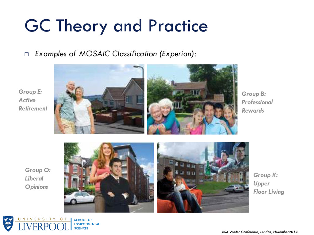
Theory and Practice Examples of MOSAIC Classification (Experian): Group B: Professional Rewards Group E: Active Retirement Group O: Liberal Opinions Group K: Upper Floor Living
Theory and Practice In general, geodemographic classifications lack a solid theory: The conceptual framework is based on a fundamental notion in social structures, homophily, which manifests spatially as a general tendency that people live in places with similar people; In nomothetic terms, the underlying clustering methodology is “simplistic” and “ambiguous”. It is true however that there is a variation of spatial autocorrelation across geographic space, for instance: Tobler's first law of geography: “everything is related to everything else, but near things are more related to distant ones” (Tobler, 1970, p. 236). Schelling's neighbourhood segregation model (Schelling, 1971). Their popularity stems from this upholding validity.
Theory and Practice Common sources of criticism: Ecological fallacy Aggregation into categorical measures smooth away high in-cluster variation. Geographic sensitivity GCs sweep away contextual differences between proximal zones - conventional techniques fail to incorporate near- geography effectively and despite the term, GCs can be in fact aspatial. Responses: Proponents claim that every GC has a particular scope and purpose – GCs are built based on the stakeholders needs and intended usage, and are construed as such. Consideration of scale, attribute selection and the availability of data: Webber, 1977: pragmatic strategy; what is deemed to work and what is required, alongside some degree of empirical evaluation. On the other hand, that view belittles the importance of the various general-purpose classifications Such debate is long withstanding, originating in the earliest of UK classifications (see Openshaw, Cullingford and Gillard, 1980 and Webber, 1980).
Outline In the regional science context, spatial socio-economic disparities have always been a crucial aspect of socio-economic research. Geodemographic “Renaissance” Geodemographics have been receiving increasing interest in the UK from the public sector, mainly driven by government pressure to demonstrate value for money and the advent of new application areas. However, national (proprietary) classifications already available may not be suitable for regional targeting: National aggregations sweep away contextual differences between proximal zones; standardizing input variables without taking into account local variation extents obscures spatial disparities and interesting patterns in finer geographic scales. Researchers without the necessary expertise may find it difficult to produce specific-purpose GCs at any given time. General-purpose classifications are more convenient to use.
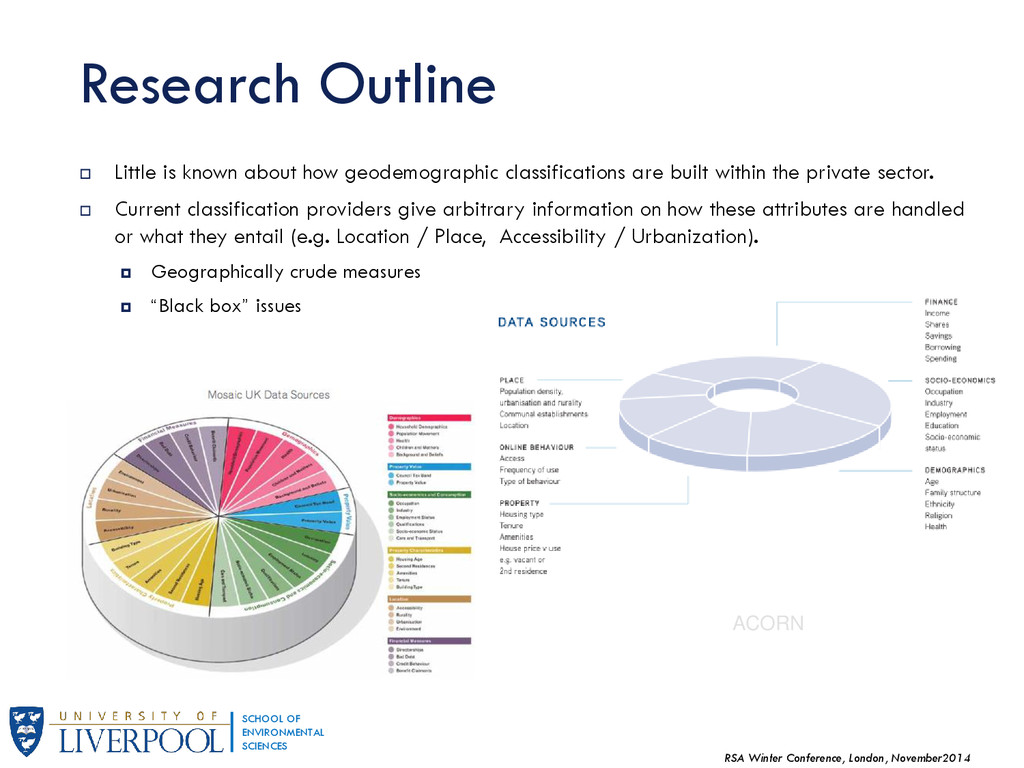
Outline Little is known about how geodemographic classifications are built within the private sector. Current classification providers give arbitrary information on how these attributes are handled or what they entail (e.g. Location / Place, Accessibility / Urbanization). Geographically crude measures “Black box” issues ACORN
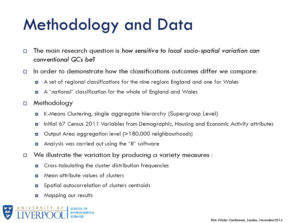
and Data The main research question is how sensitive to local socio-spatial variation can conventional GCs be? In order to demonstrate how the classifications outcomes differ we compare: A set of regional classifications for the nine regions England and one for Wales A “national” classification for the whole of England and Wales Methodology K-Means Clustering, single aggregate hierarchy (Supergroup Level) Initial 67 Census 2011 Variables from Demographic, Housing and Economic Activity attributes Output Area aggregation level (>180.000 neighbourhoods) Analysis was carried out using the “R” software We illustrate the variation by producing a variety measures : Cross-tabulating the cluster distribution frequencies Mean attribute values of clusters Spatial autocorrelation of clusters centroids Mapping our results
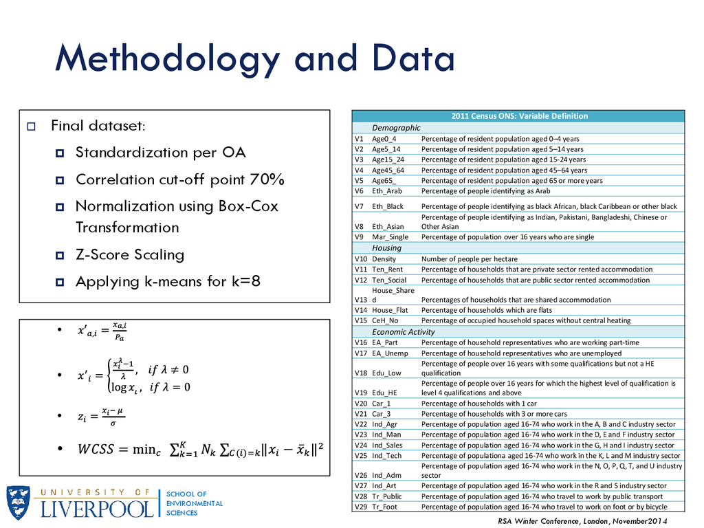
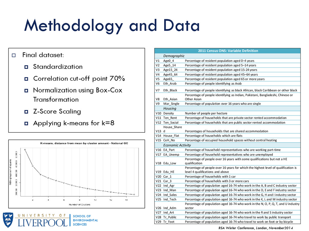
and Data Final dataset: Standardization per OA Correlation cut-off point 70% Normalization using Box-Cox Transformation Z-Score Scaling Applying k-means for k=8 2011 Census ONS: Variable Definition Demographic V1 Age0_4 Percentage of resident population aged 0–4 years V2 Age5_14 Percentage of resident population aged 5–14 years V3 Age15_24 Percentage of resident population aged 15-24 years V4 Age45_64 Percentage of resident population aged 45–64 years V5 Age65_ Percentage of resident population aged 65 or more years V6 Eth_Arab Percentage of people identifying as Arab V7 Eth_Black Percentage of people identifying as black African, black Caribbean or other black V8 Eth_Asian Percentage of people identifying as Indian, Pakistani, Bangladeshi, Chinese or Other Asian V9 Mar_Single Percentage of population over 16 years who are single Housing V10 Density Number of people per hectare V11 Ten_Rent Percentage of households that are private sector rented accommodation V12 Ten_Social Percentage of households that are public sector rented accommodation V13 House_Share d Percentages of households that are shared accommodation V14 House_Flat Percentage of households which are flats V15 CeH_No Percentage of occupied household spaces without central heating Economic Activity V16 EA_Part Percentage of household representatives who are working part-time V17 EA_Unemp Percentage of household representatives who are unemployed V18 Edu_Low Percentage of people over 16 years with some qualifications but not a HE qualification V19 Edu_HE Percentage of people over 16 years for which the highest level of qualification is level 4 qualifications and above V20 Car_1 Percentage of households with 1 car V21 Car_3 Percentage of households with 3 or more cars V22 Ind_Agr Percentage of population aged 16-74 who work in the A, B and C industry sector V23 Ind_Man Percentage of population aged 16-74 who work in the D, E and F industry sector V24 Ind_Sales Percentage of population aged 16-74 who work in the G, H and I industry sector V25 Ind_Tech Percentage of populationa aged 16-74 who work in the K, L and M industry sector V26 Ind_Adm Percentage of population aged 16-74 who work in the N, O, P, Q, T, and U industry sector V27 Ind_Art Percentage of population aged 16-74 who work in the R and S industry sector V28 Tr_Public Percentage of population aged 16-74 who travel to work by public transport V29 Tr_Foot Percentage of population aged 16-74 who travel to work on foot or by bicycle
and Data Final dataset: Standardization Correlation cut-off point 70% Normalization using Box-Cox Transformation Z-Score Scaling Applying k-means for k=8 2011 Census ONS: Variable Definition Demographic V1 Age0_4 Percentage of resident population aged 0–4 years V2 Age5_14 Percentage of resident population aged 5–14 years V3 Age15_24 Percentage of resident population aged 15-24 years V4 Age45_64 Percentage of resident population aged 45–64 years V5 Age65_ Percentage of resident population aged 65 or more years V6 Eth_Arab Percentage of people identifying as Arab V7 Eth_Black Percentage of people identifying as black African, black Caribbean or other black V8 Eth_Asian Percentage of people identifying as Indian, Pakistani, Bangladeshi, Chinese or Other Asian V9 Mar_Single Percentage of population over 16 years who are single Housing V10 Density Number of people per hectare V11 Ten_Rent Percentage of households that are private sector rented accommodation V12 Ten_Social Percentage of households that are public sector rented accommodation V13 House_Share d Percentages of households that are shared accommodation V14 House_Flat Percentage of households which are flats V15 CeH_No Percentage of occupied household spaces without central heating Economic Activity V16 EA_Part Percentage of household representatives who are working part-time V17 EA_Unemp Percentage of household representatives who are unemployed V18 Edu_Low Percentage of people over 16 years with some qualifications but not a HE qualification V19 Edu_HE Percentage of people over 16 years for which the highest level of qualification is level 4 qualifications and above V20 Car_1 Percentage of households with 1 car V21 Car_3 Percentage of households with 3 or more cars V22 Ind_Agr Percentage of population aged 16-74 who work in the A, B and C industry sector V23 Ind_Man Percentage of population aged 16-74 who work in the D, E and F industry sector V24 Ind_Sales Percentage of population aged 16-74 who work in the G, H and I industry sector V25 Ind_Tech Percentage of population aged 16-74 who work in the K, L and M industry sector V26 Ind_Adm Percentage of population aged 16-74 who work in the N, O, P, Q, T, and U industry sector V27 Ind_Art Percentage of population aged 16-74 who work in the R and S industry sector V28 Tr_Public Percentage of population aged 16-74 who travel to work by public transport V29 Tr_Foot Percentage of population aged 16-74 who travel to work on foot or by bicycle
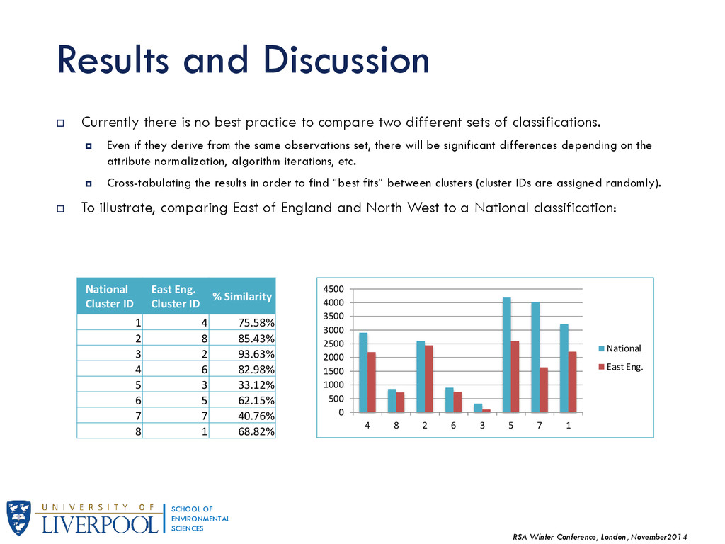
Currently there is no best practice to compare two different sets of classifications. Even if they derive from the same observations set, there will be significant differences depending on the attribute normalization, algorithm iterations, etc. Cross-tabulating the results in order to find “best fits” between clusters (cluster IDs are assigned randomly). To illustrate, comparing East of England and North West to a National classification: Results and Discussion National Cluster ID East Eng. Cluster ID % Similarity 1 4 75.58% 2 8 85.43% 3 2 93.63% 4 6 82.98% 5 3 33.12% 6 5 62.15% 7 7 40.76% 8 1 68.82% 0 500 1000 1500 2000 2500 3000 3500 4000 4500 4 8 2 6 3 5 7 1 National East Eng.
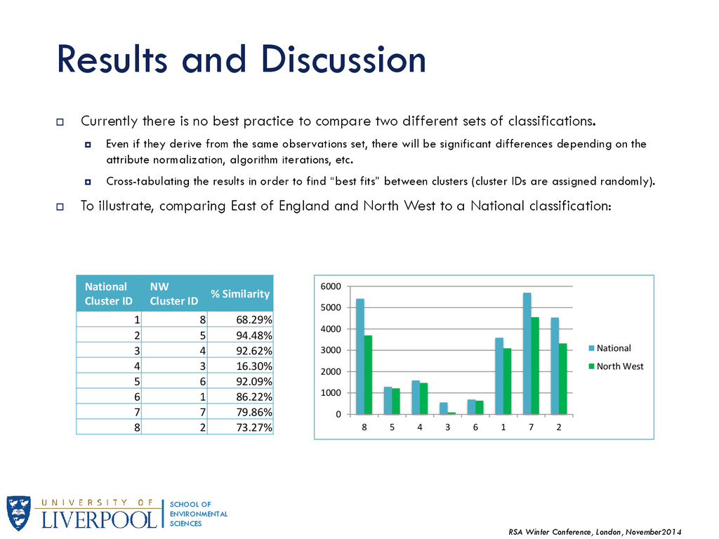
Currently there is no best practice to compare two different sets of classifications. Even if they derive from the same observations set, there will be significant differences depending on the attribute normalization, algorithm iterations, etc. Cross-tabulating the results in order to find “best fits” between clusters (cluster IDs are assigned randomly). To illustrate, comparing East of England and North West to a National classification: Results and Discussion National Cluster ID NW Cluster ID % Similarity 1 8 68.29% 2 5 94.48% 3 4 92.62% 4 3 16.30% 5 6 92.09% 6 1 86.22% 7 7 79.86% 8 2 73.27% 0 1000 2000 3000 4000 5000 6000 8 5 4 3 6 1 7 2 National North West
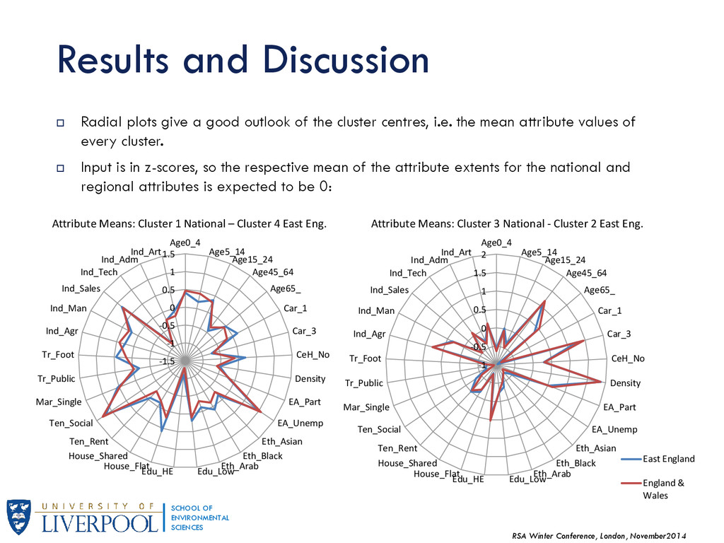
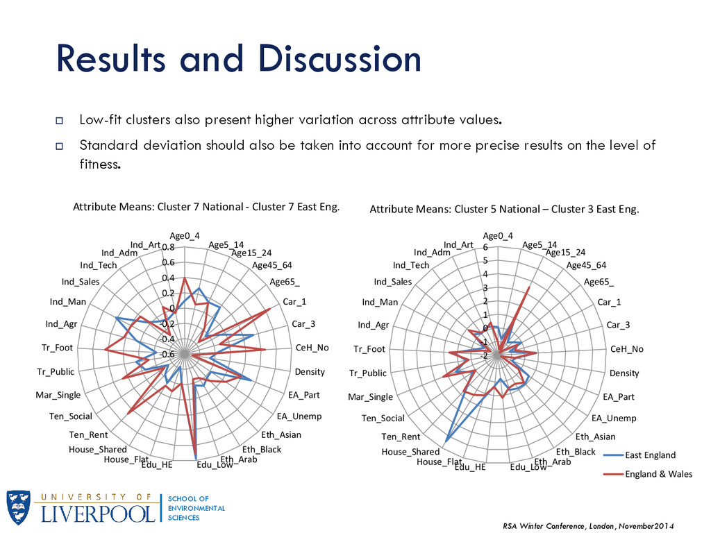
Radial plots give a good outlook of the cluster centres, i.e. the mean attribute values of every cluster. Input is in z-scores, so the respective mean of the attribute extents for the national and regional attributes is expected to be 0: Results and Discussion -1.5 -1 -0.5 0 0.5 1 1.5 Age0_4 Age5_14 Age15_24 Age45_64 Age65_ Car_1 Car_3 CeH_No Density EA_Part EA_Unemp Eth_Asian Eth_Black Eth_Arab Edu_Low Edu_HE House_Flat House_Shared Ten_Rent Ten_Social Mar_Single Tr_Public Tr_Foot Ind_Agr Ind_Man Ind_Sales Ind_Tech Ind_Adm Ind_Art Attribute Means: Cluster 1 National – Cluster 4 East Eng. -1 -0.5 0 0.5 1 1.5 2 Age0_4 Age5_14 Age15_24 Age45_64 Age65_ Car_1 Car_3 CeH_No Density EA_Part EA_Unemp Eth_Asian Eth_Black Eth_Arab Edu_Low Edu_HE House_Flat House_Shared Ten_Rent Ten_Social Mar_Single Tr_Public Tr_Foot Ind_Agr Ind_Man Ind_Sales Ind_Tech Ind_Adm Ind_Art Attribute Means: Cluster 3 National - Cluster 2 East Eng. East England England & Wales
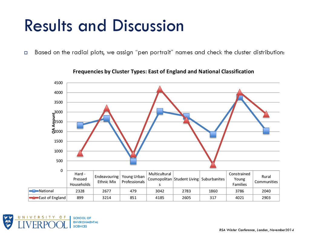
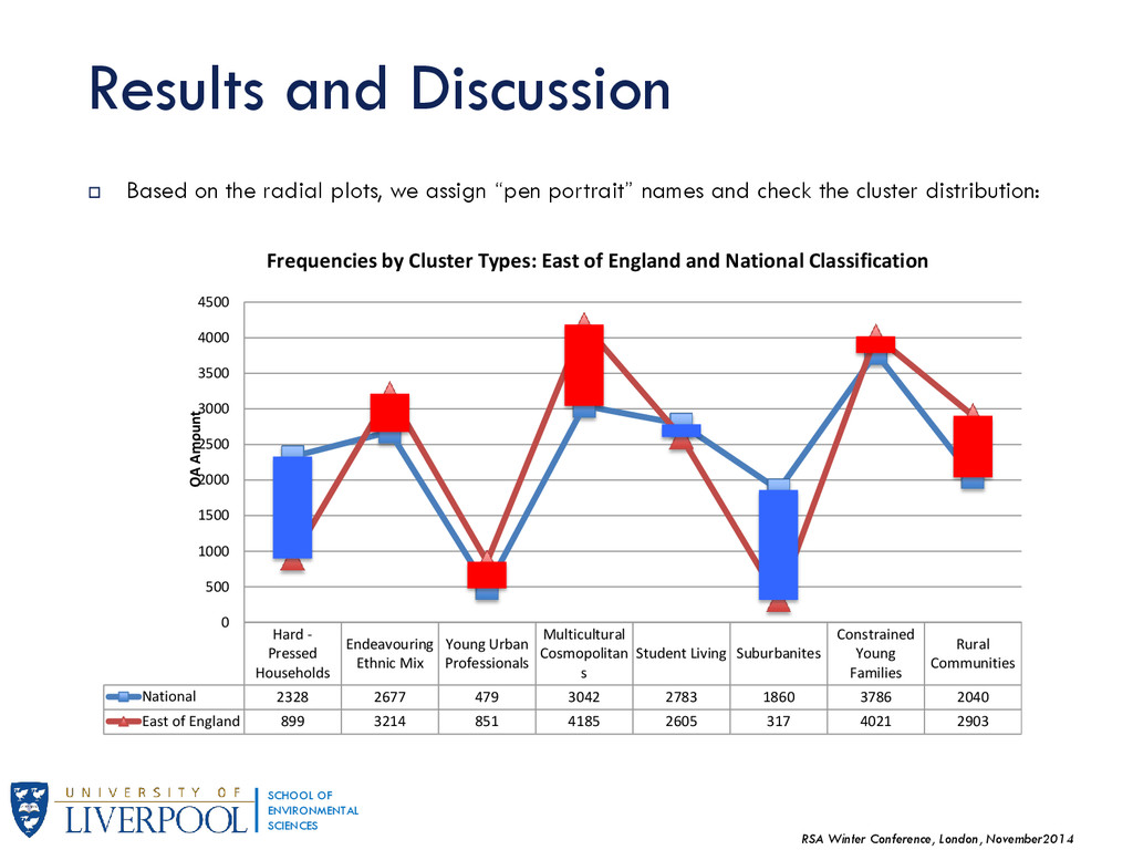
Based on the radial plots, we assign “pen portrait” names and check the cluster distribution: Hard - Pressed Households Endeavouring Ethnic Mix Young Urban Professionals Multicultural Cosmopolitan s Student Living Suburbanites Constrained Young Families Rural Communities National 2328 2677 479 3042 2783 1860 3786 2040 East of England 899 3214 851 4185 2605 317 4021 2903 0 500 1000 1500 2000 2500 3000 3500 4000 4500 OA Amount Frequencies by Cluster Types: East of England and National Classification Results and Discussion
Based on the radial plots, we assign “pen portrait” names and check the cluster distribution: Results and Discussion Hard - Pressed Households Endeavouring Ethnic Mix Young Urban Professionals Multicultural Cosmopolitan s Student Living Suburbanites Constrained Young Families Rural Communities National 2328 2677 479 3042 2783 1860 3786 2040 East of England 899 3214 851 4185 2605 317 4021 2903 0 500 1000 1500 2000 2500 3000 3500 4000 4500 OA Amount Frequencies by Cluster Types: East of England and National Classification
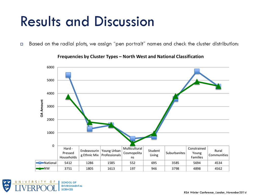
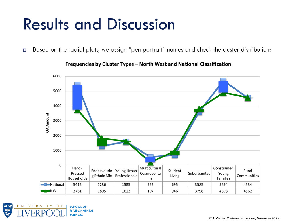
Based on the radial plots, we assign “pen portrait” names and check the cluster distribution: Hard - Pressed Households Endeavourin g Ethnic Mix Young Urban Professionals Multicultural Cosmopolita ns Student Living Suburbanites Constrained Young Families Rural Communities National 5412 1286 1585 552 695 3585 5694 4534 NW 3751 1805 1613 197 946 3798 4898 4562 0 1000 2000 3000 4000 5000 6000 OA Amount Frequencies by Cluster Types – North West and National Classification Results and Discussion
Based on the radial plots, we assign “pen portrait” names and check the cluster distribution: Hard - Pressed Households Endeavourin g Ethnic Mix Young Urban Professionals Multicultural Cosmopolita ns Student Living Suburbanites Constrained Young Families Rural Communities National 5412 1286 1585 552 695 3585 5694 4534 NW 3751 1805 1613 197 946 3798 4898 4562 0 1000 2000 3000 4000 5000 6000 OA Amount Frequencies by Cluster Types – North West and National Classification Results and Discussion
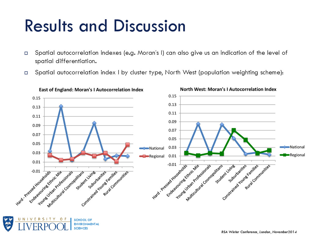
Spatial autocorrelation indexes (e.g. Moran’s I) can also give us an indication of the level of spatial differentiation. Spatial autocorrelation index I by cluster type, North West (population weighting scheme): Results and Discussion -0.01 0.01 0.03 0.05 0.07 0.09 0.11 0.13 0.15 East of England: Moran's I Autocorrelation Index National Regional -0.01 0.01 0.03 0.05 0.07 0.09 0.11 0.13 0.15 North West: Moran's I Autocorrelation Index National Regional
and Discussion These preliminary results show some level of differentiation between regional and national level classification, validating the initial hypothesis that caution should be taken when using conventional national classifications for local area analyses. The traditional “aspatial” approach has a number of implications: For marketing related applications of geodemographics, a lack of local sensitivity may have fiscal implications, such as a reduced uptake of a product or service. In public sector uses, the consequences may be more severe, with mistargeting having potential implications on life chances, health and wellbeing. Another way to address these issues is with bottom-up approaches in clustering algorithms compared to top-down: The process of adding smaller classifications to a larger one can provide a classification frameworks that accounts better for local area geography. However issues arise as cluster type and/or amount of smaller classifications may not correspond properly across regions. The extent of “near-geography” cannot be clearly defined and current practices (mostly private sector) are geographically “crude” (arbitrary zones or administrative boundaries that may not correspond with the organizations of actual communities).
and Discussion On the other hand it could be argued that disaggregated regional classifications may loose those practical benefits associated with classifications created for national extents (comparative opportunities, correlations with other national survey estimates, etc). Signs of growth in the regional data stores (e.g. http://data.london.gov.uk/) which can overcome such limitations, as further small area descriptor data become available; Regional classifications also offer the potential to develop non-census based or intra-census classifications. Future research is needed to produce measures of near geography that can capture such associations and evaluate them vis-à-vis traditional geodemographic models.
London, November 2014 Acknowledgements: This work is funded as part of an ESRC PhD studentship and is in collaboration with the Office for National Statistics
![Thank you for your time [email protected] RSA Winter Conference –](https://files.speakerdeck.com/presentations/ba71c5205d010132feb0261f207a90b3/slide_26.jpg)