Share
Embed
Hydroacoustic signatures of riverbed sediments using multibeam sonar
Presented at SEDHYD 2015, Reno, Nevada
Daniel Buscombe
April 02, 2015
Transcript
45 slides
-
Aim: mapping of Colorado River bed sediments. Why? Where is
the sand? Habitats Geomorphology -
Aim: mapping of Colorado River bed sediments. Why? How much
sand is there? Budgets Sediment transport models -
Aim: mapping of Colorado River bed sediments. Why? How does
that vary in time? Dam operations Experimental high flows -
Bed sediments sampled using video ... ... which has revealed
enormous bed sediment heterogeneity Fine sand through to boulders Abrupt transitions -
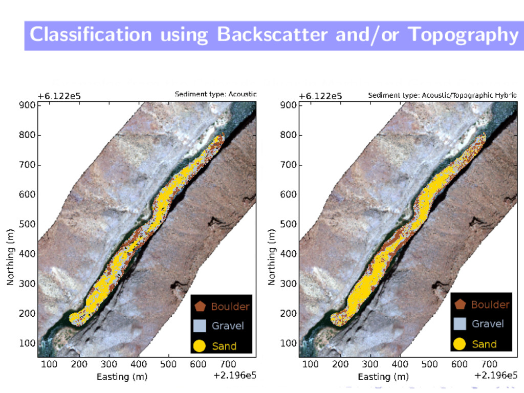
Objectives. Infer bed sediments using high-frequency backscatter and topography Develop
a data-driven approach using patches of known sediment type Has to fit into existing channel mapping protocol -
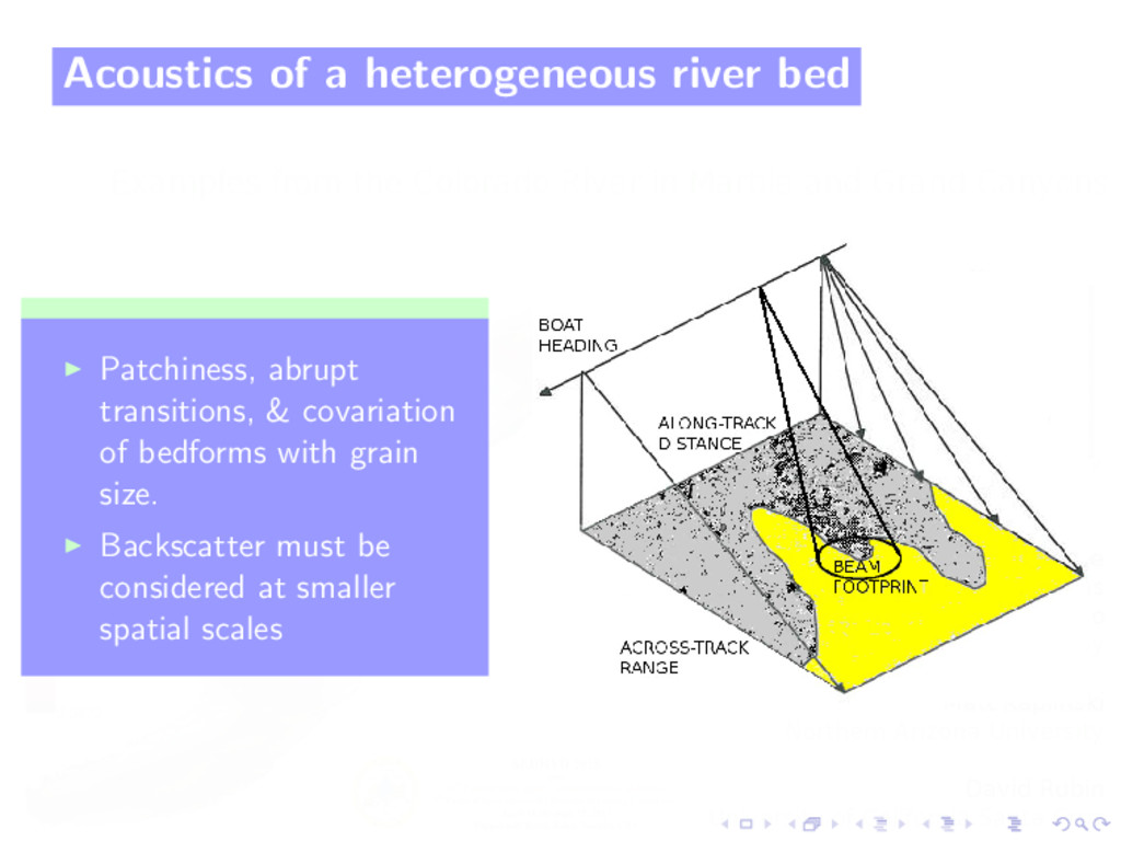
Acoustics of a heterogeneous river bed Patchiness, abrupt transitions, &
covariation of bedforms with grain size. Backscatter must be considered at smaller spatial scales -
Stochastic geometry. 1) Spectral Strength P1(K) = ω1 (h0|K|)γ1 measure
of power at low frequencies -
Stochastic geometry. 2) Spectral Width P1(K) = ω1 (h0|K|) γ1
measure of the rate of decay in power as a function of increasing frequency. -
Stochastic geometry. 3) Spectral Variance σ2 1 = 2 K0
P1(K)dK overall power in the spectrum over all frequencies -
Relationship between sediment type & spectral strength Low-frequency component increases
with increasing clast size Strong relationships with roughness -
Relationship between sediment type & ‘roughness’ Variance in fluctuating part
of both the topographic and backscatter signal increase with increasing clast size -
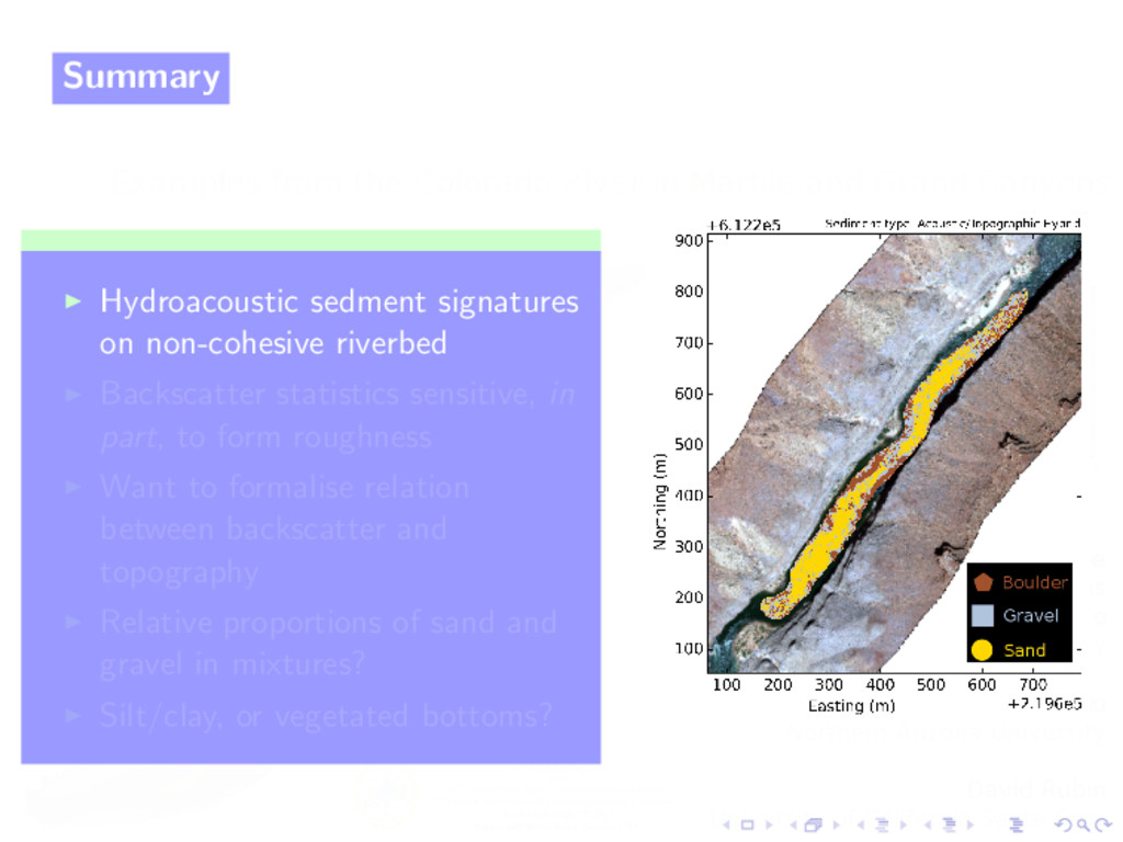
Summary Hydroacoustic sedment signatures on non-cohesive riverbed Backscatter statistics sensitive,
in part, to form roughness Want to formalise relation between backscatter and topography Relative proportions of sand and gravel in mixtures? Silt/clay, or vegetated bottoms? -
Summary Hydroacoustic sedment signatures on non-cohesive riverbed Backscatter statistics sensitive,
in part, to form roughness Want to formalise relation between backscatter and topography Relative proportions of sand and gravel in mixtures? Silt/clay, or vegetated bottoms? -
Summary Hydroacoustic sedment signatures on non-cohesive riverbed Backscatter statistics sensitive,
in part, to form roughness Want to formalise relation between backscatter and topography Relative proportions of sand and gravel in mixtures? Silt/clay, or vegetated bottoms? -
Summary Hydroacoustic sedment signatures on non-cohesive riverbed Backscatter statistics sensitive,
in part, to form roughness Want to formalise relation between backscatter and topography Relative proportions of sand and gravel in mixtures? Silt/clay, or vegetated bottoms? Sandy gravels in Glen Canyon, Dec 2014 -
Summary Hydroacoustic sedment signatures on non-cohesive riverbed Backscatter statistics sensitive,
in part, to form roughness Want to formalise relation between backscatter and topography Relative proportions of sand and gravel in mixtures? Silt/clay, or vegetated bottoms? -
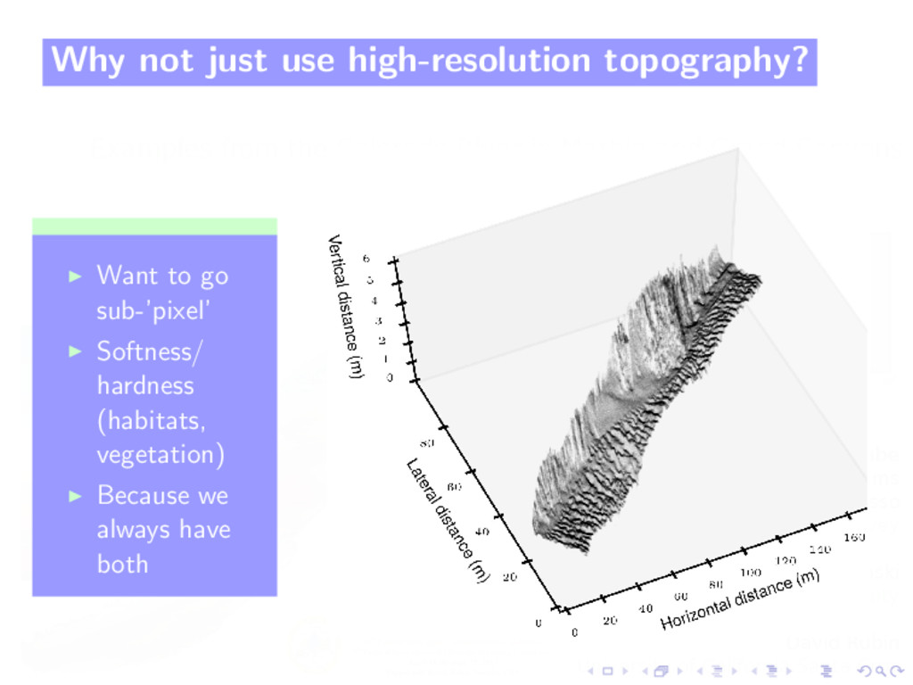
Why not just use high-resolution topography? Want to go sub-’pixel’
Softness/ hardness (habitats, vegetation) Because we always have both -
Acoustics of a River Bed Fall between two scattering regimes
depending on grain size -
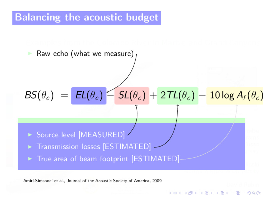
Balancing the acoustic budget Raw echo (what we measure) BS(θc
) = EL(θc ) − SL(θc ) + 2TL(θc ) − 10 log Af (θc ) Source level [MEASURED] Transmission losses [ESTIMATED] True area of beam footprint [ESTIMATED] Amiri-Simkooei et al., Journal of the Acoustic Society of America, 2009 -
Balancing the acoustic budget Raw echo (what we measure) BS(θc
) = EL(θc ) − SL(θc ) + 2TL(θc ) − 10 log Af (θc ) Source level [MEASURED] Transmission losses [ESTIMATED] True area of beam footprint [ESTIMATED] Amiri-Simkooei et al., Journal of the Acoustic Society of America, 2009 -
Balancing the acoustic budget Raw echo (what we measure) BS(θc
) = EL(θc ) − SL(θc ) + 2TL(θc ) − 10 log Af (θc ) Source level [MEASURED] Transmission losses [ESTIMATED] True area of beam footprint [ESTIMATED] Amiri-Simkooei et al., Journal of the Acoustic Society of America, 2009 -
Balancing the acoustic budget Raw echo (what we measure) BS(θc
) = EL(θc ) − SL(θc ) + 2TL(θc ) − 10 log Af (θc ) Source level [MEASURED] Transmission losses [ESTIMATED] True area of beam footprint [ESTIMATED] Amiri-Simkooei et al., Journal of the Acoustic Society of America, 2009 -
Transmission, amplification & sampling BS(θc ) = EL(θc ) −
SL(θc ) + 2TL(θc ) − 10 log Af (θc ) Function of: Output power [MEASURED] Input amplification [MEASURED] Ping rate [MEASURED] Pulse length [MEASURED] -
Water & sediment attenuation BS(θc ) = EL(θc ) −
SL(θc ) + 2TL(θc ) − 10 log Af (θc ) Sediment attenuation [ESTIMATED] using Urick (1948): Particle size and concentration [MEASURED] Particle density [ESTIMATED] Homogeneous mixing [ASSUMED] Water attenuation [ESTIMATED] using Fisher & Simmons (1977): Temperature [MEASURED] Salinity & pH [ESTIMATED] Homogeneous mixing [ASSUMED] Fisher and Simmons. Journal of the Acoustic Society of America, 1977. Urick. Journal of the Acoustic Society of America, 1948. -
Beam footprint BS(θc ) = EL(θc ) − SL(θc )
+ 2TL(θc ) − 10 log Af (θc ) Function of: Across- & along-track slopes [ESTIMATED] Angular range [ESTIMATED] Ping rate [MEASURED] Grazing angle (ψc ) [ESTIMATED] -
Pre-Processing Correct by mean amplitude per grazing angle Outside nadir
region, averaging over neighbouring bins Subtracted then value at reference angle (30o) is added back in -
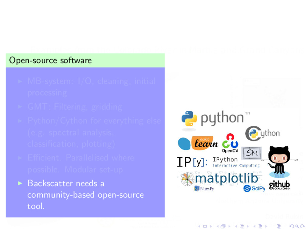
Software Open-source software MB-system: I/O, cleaning, initial processing GMT: Filtering,
gridding Python/Cython for everything else (e.g. spectral analysis, classification, plotting) Efficient. Parallelised where possible. Modular set-up Backscatter needs a community-based open-source tool. Caress and Chayes. Proceedings of the IEEE Oceans 95 Conference, 1995. Caress and Chayes. Marine Geophysical Research, 2006. -
Software Open-source software MB-system: I/O, cleaning, initial processing GMT: Filtering,
gridding Python/Cython for everything else (e.g. spectral analysis, classification, plotting) Efficient. Parallelised where possible. Modular set-up Backscatter needs a community-based open-source tool. Wessel et al. EOS Trans. AGU, 1991, 1995, 1998, 2013 -
Software Open-source software MB-system: I/O, cleaning, initial processing GMT: Filtering,
gridding Python/Cython for everything else (e.g. spectral analysis, classification, plotting) Efficient. Parallelised where possible. Modular set-up Backscatter needs a community-based open-source tool. -
Software Open-source software MB-system: I/O, cleaning, initial processing GMT: Filtering,
gridding Python/Cython for everything else (e.g. spectral analysis, classification, plotting) Efficient. Parallelised where possible. Modular set-up Backscatter needs a community-based open-source tool. -
Software Open-source software MB-system: I/O, cleaning, initial processing GMT: Filtering,
gridding Python/Cython for everything else (e.g. spectral analysis, classification, plotting) Efficient. Parallelised where possible. Modular set-up Backscatter needs a community-based open-source tool.