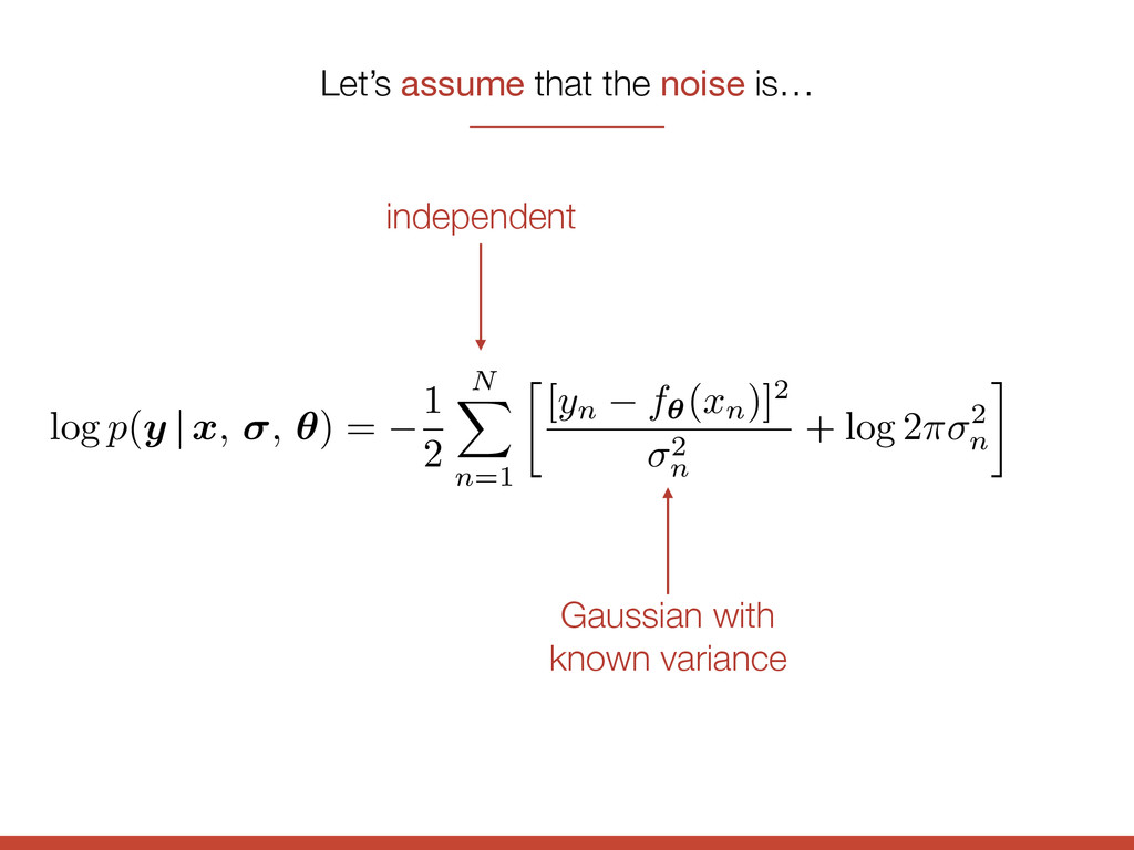
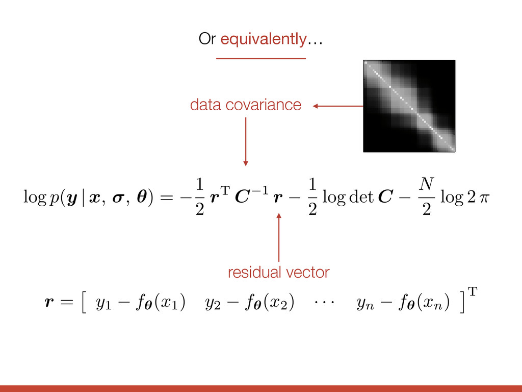
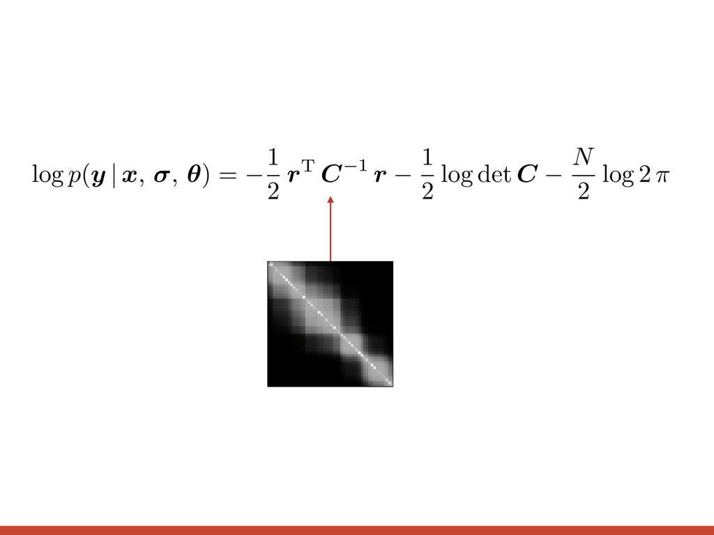
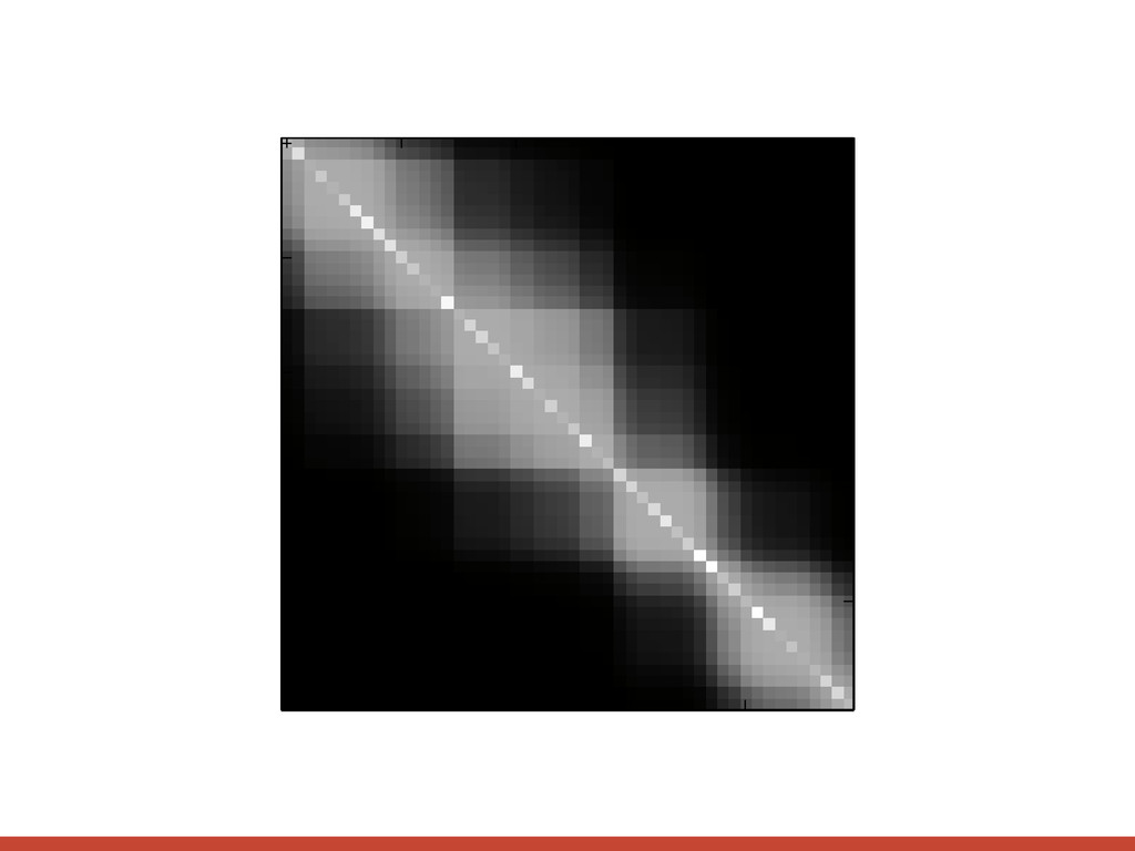
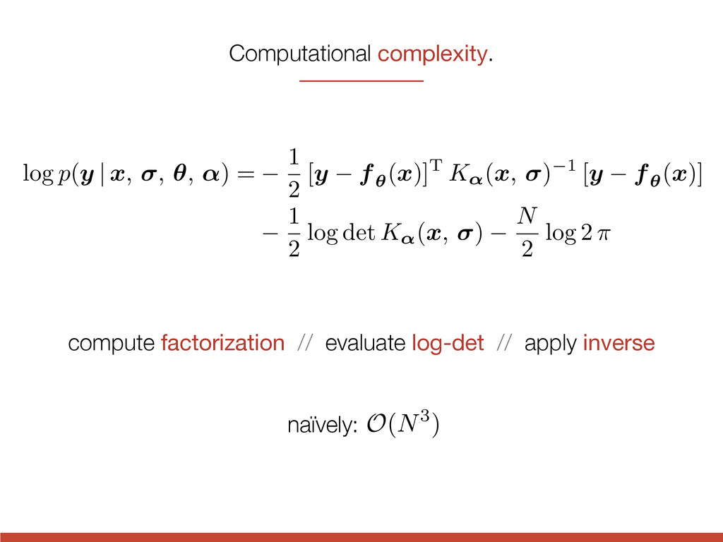
2 r T C 1 r 1 2 log det C N 2 log 2 ⇡ Or equivalently… data covariance residual vector r = ⇥ y1 f✓( x1) y2 f✓( x2) · · · yn f✓( xn) ⇤T 0 10 20 30 40 0 10 20 30 40
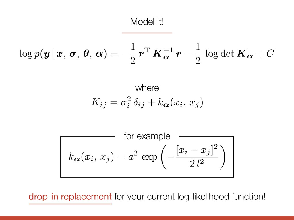
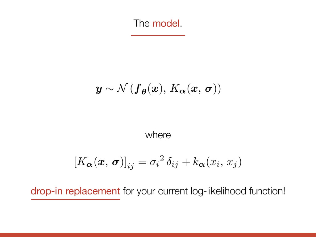
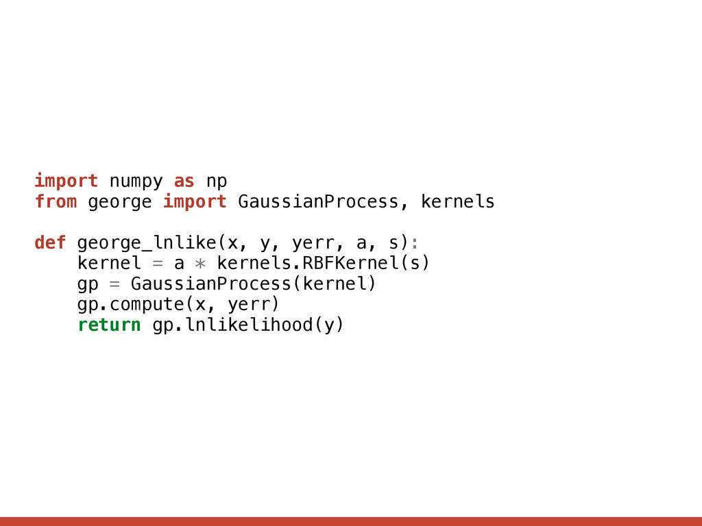
, ↵) = 1 2 r T K 1 ↵ r 1 2 log det K↵ + C k↵(xi, xj) = a 2 exp ✓ [xi xj] 2 2 l 2 ◆ for example Kij = 2 i ij + k↵( xi, xj) where drop-in replacement for your current log-likelihood function!
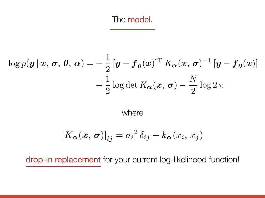
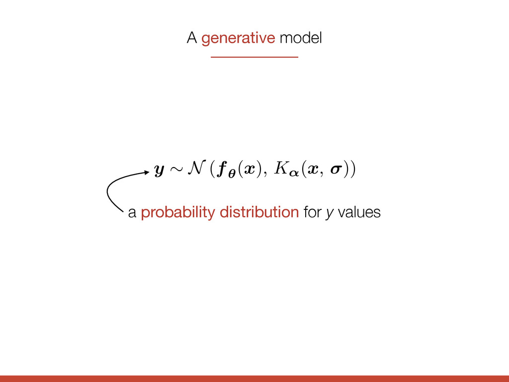
= 1 2 [y f✓(x)] T K↵(x , ) 1 [y f✓(x)] 1 2 log det K↵(x , ) N 2 log 2 ⇡ where The model. drop-in replacement for your current log-likelihood function! [ K↵( x, )]ij = i 2 ij + k↵( xi, xj)
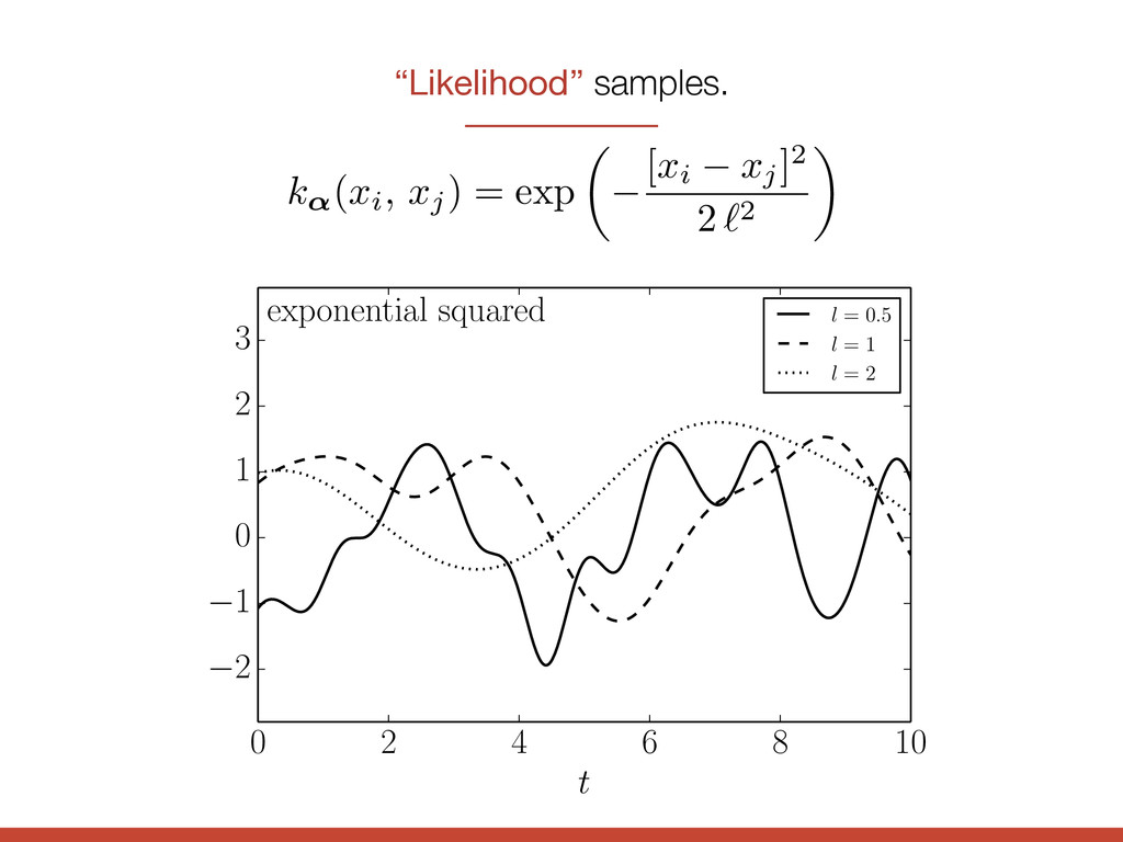
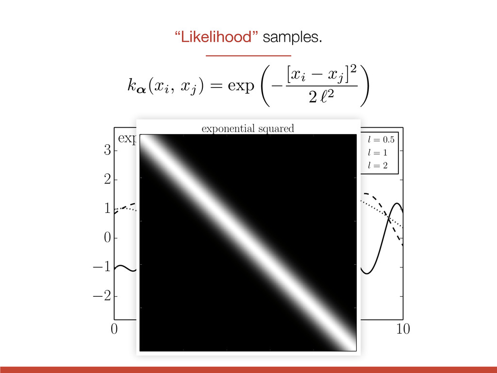
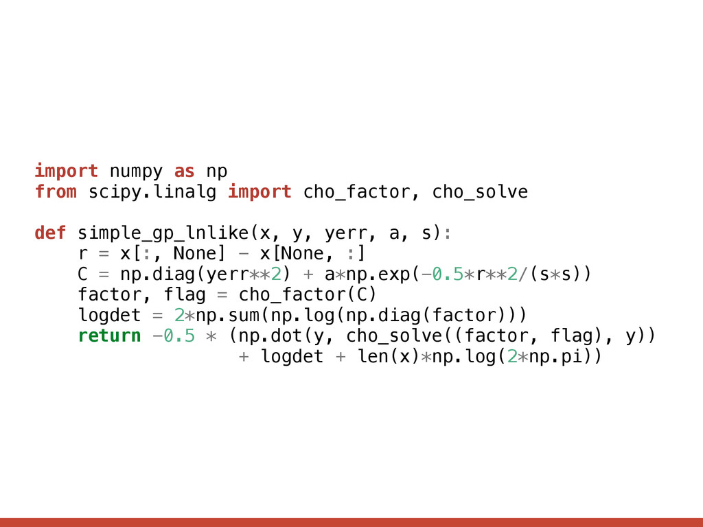
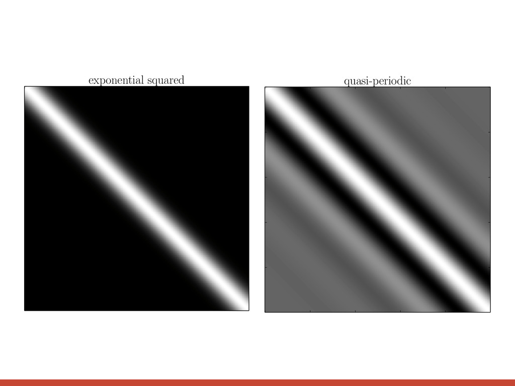
l = 0.5 l = 1 l = 2 3 quasi-periodic l = 2, P = 3 l = 3, P = 3 l = 3, P = 1 2 1 0 1 0 2 4 6 8 10 t 2 1 0 1 2 3 quasi-periodic l = 2, P = 3 l = 3, P = 3 l = 3, P = 1 k↵(xi, xj) = exp ✓ [xi xj] 2 2 ` 2 ◆
l = 0.5 l = 1 l = 2 3 quasi-periodic l = 2, P = 3 l = 3, P = 3 l = 3, P = 1 2 1 0 1 0 2 4 6 8 10 t 2 1 0 1 2 3 quasi-periodic l = 2, P = 3 l = 3, P = 3 l = 3, P = 1 exponential squared k↵(xi, xj) = exp ✓ [xi xj] 2 2 ` 2 ◆
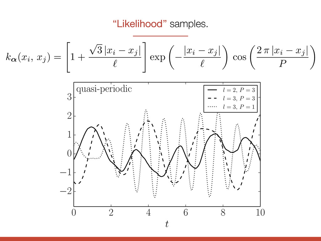
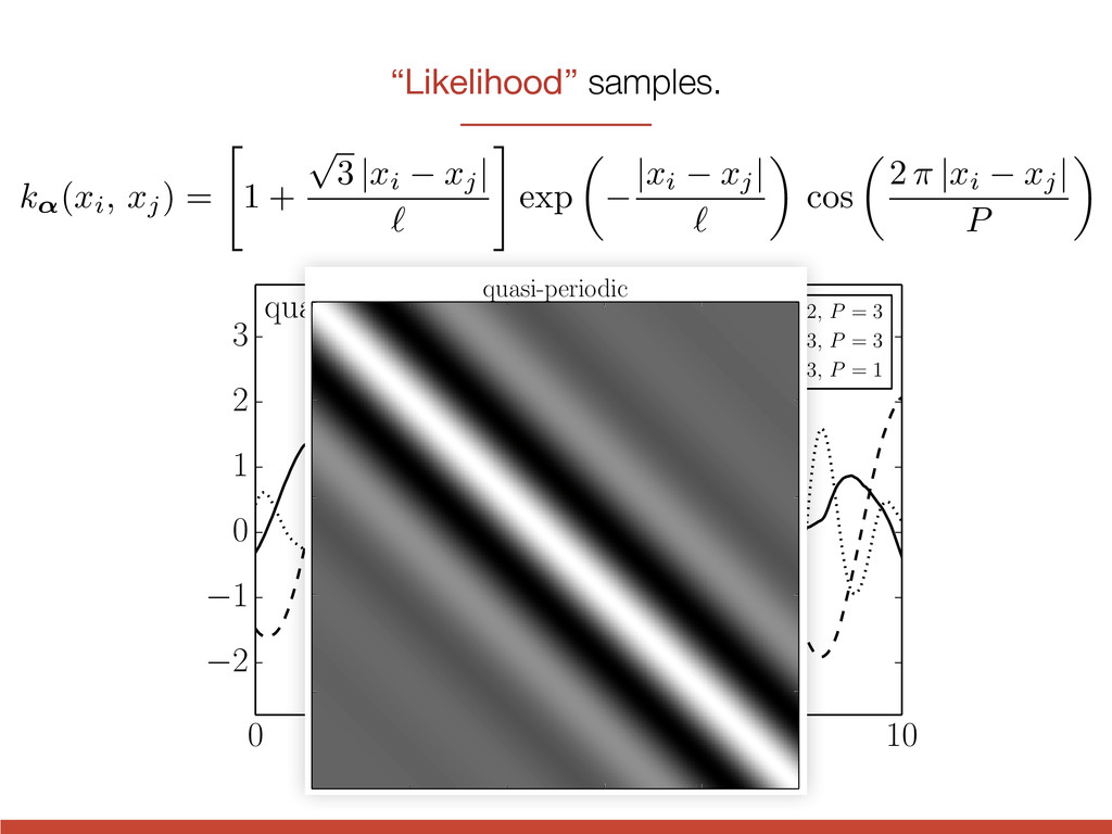
8 10 t 2 1 0 1 2 3 quasi-periodic l = 2, P = 3 l = 3, P = 3 l = 3, P = 1 k↵(xi, xj) = " 1 + p 3 | xi xj | ` # exp ✓ | xi xj | ` ◆ cos ✓ 2 ⇡ | xi xj | P ◆
8 10 t 2 1 0 1 2 3 quasi-periodic l = 2, P = 3 l = 3, P = 3 l = 3, P = 1 quasi-periodic k↵(xi, xj) = " 1 + p 3 | xi xj | ` # exp ✓ | xi xj | ` ◆ cos ✓ 2 ⇡ | xi xj | P ◆
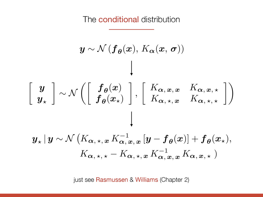
), K↵( x , )) y y? ⇠ N ✓ f✓ ( x ) f✓ ( x?) , K ↵ , x , x K ↵ , x , ? K ↵ , ?, x K ↵ , ?, ? ◆ y? | y ⇠ N K ↵ , ?, x K 1 ↵ , x , x [ y f✓ ( x )] + f✓ ( x?), K ↵ , ?, ? K ↵ , ?, x K 1 ↵ , x , x K ↵ , x , ? ) just see Rasmussen & Williams (Chapter 2)
![635 640 645 650 655 660 time [KBJD] 0.004 0.003](https://files.speakerdeck.com/presentations/36035540d602013172e21e3c4e84372f/slide_11.jpg)
![460 480 500 520 time [KBJD] 0.015 0.010 0.005 0.000](https://files.speakerdeck.com/presentations/36035540d602013172e21e3c4e84372f/slide_14.jpg)
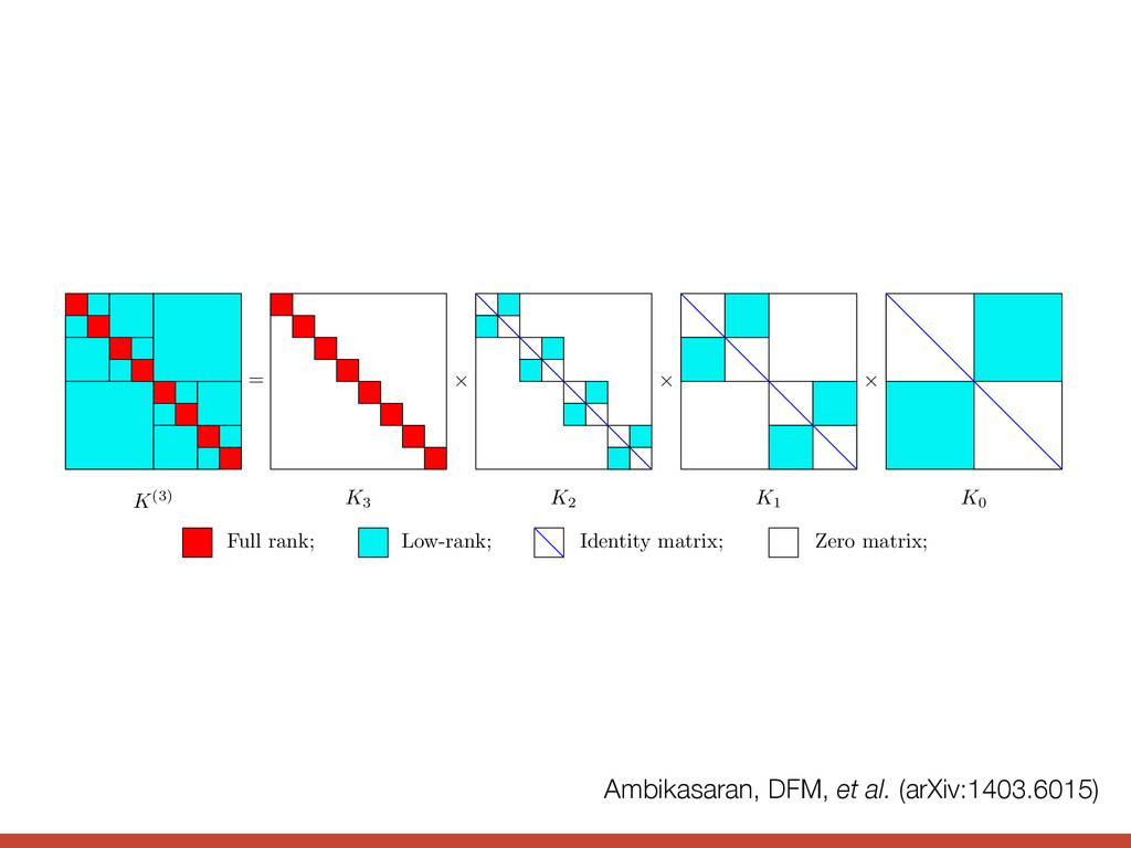
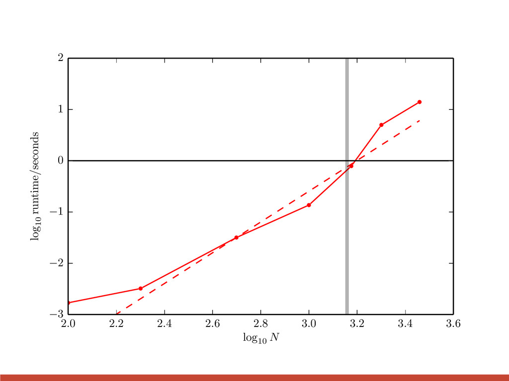
![time [days] Ambikasaran, DFM, et al. (arXiv:1403.6015)](https://files.speakerdeck.com/presentations/36035540d602013172e21e3c4e84372f/slide_82.jpg)
![Resources gaussianprocess.org/gpml github.com/dfm/ gp george [email protected]](https://files.speakerdeck.com/presentations/36035540d602013172e21e3c4e84372f/slide_92.jpg)