Hierarchical inference for exoplanet populations

My slides for #iau2015

Transcript

1. Hierarchical inference for exoplanet populations Dan Foreman-Mackey (Sagan Fellow, U. Washington) iau exostats / 2015-08-03
2. Probabilistic modeling for exoplanet populations Dan Foreman-Mackey (Sagan Fellow, U. Washington) iau exostats / 2015-08-03
3. "backup Hogg" Credit: Christopher Stumm
4. "backup Hogg" Dan Foreman-Mackey Sagan Fellow, University of Washington dfm.io / @exoplaneteer / github.com/dfm
5. summary ▶︎ hierarchical inference and probabilistic modeling provide a consistent framework for: ▶︎ measurement uncertainties ▶︎ missing data ▶︎ heterogeneous datasets ▶︎ false positives/alarms ▶︎ ...
6. summary ▶︎ hierarchical inference and probabilistic modeling provide a consistent framework for: ▶︎ measurement uncertainties ▶︎ missing data ▶︎ heterogeneous datasets ▶︎ false positives/alarms ▶︎ ... ▶︎ it isn't hard
7. population inference ▶︎ population: global distribution and rate of physical parameters (period, mass, multiplicity, etc.) ▶︎ inference: coming to a conclusion based on evidence
8. population inference ▶︎ what can we say about the population of exoplanets based on the existing set of large, heterogeneous datasets?
9. physics data
10. physics data !!!!
11. population inference ▶︎ what can we say about the population of exoplanets based on the full set of photons detected by Kepler, Keck, GPI, [your favorite instrument here], etc.?
12. THAT'S IMPOSSIBLE
13. hierarchical inference (hierarchical Bayesian modeling) ▶︎ hierarchical inference: exploit structure in the problem to make it tractable
14. hierarchical inference (hierarchical Bayesian modeling) ▶︎ we do this already!
15. physics data !!!!
16. population planetary systems data
17. population planetary systems data physics
18. k = 1, · · · , K ✓ wk xk per-object parameters (period, radius, etc.) per-object observations global population
19. p({ xk } | ✓ ) = Z p({ xk }, { wk } | ✓ ) d{ wk } = Z p({ xk } | { wk }) p({ wk } | ✓ ) d{ wk } the Big Integral™
20. solving the Big Integral™ ▶︎ for small problems, use available tools like JAGS, Stan, PyMC, emcee, etc. ▶︎ for bigger problems, you'll probably need something problem specific
21. SO WHAT?!
22. an example: Kepler ▶︎ what can we say about the joint period– radius distribution based on the Kepler dataset?
23. 101 102 orbital period [days] 100 101 planet radius [R ] Data from: The Exoplanet Archive typical error bar
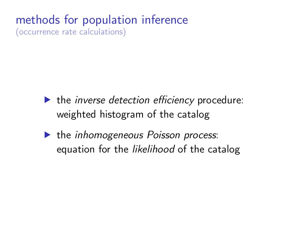
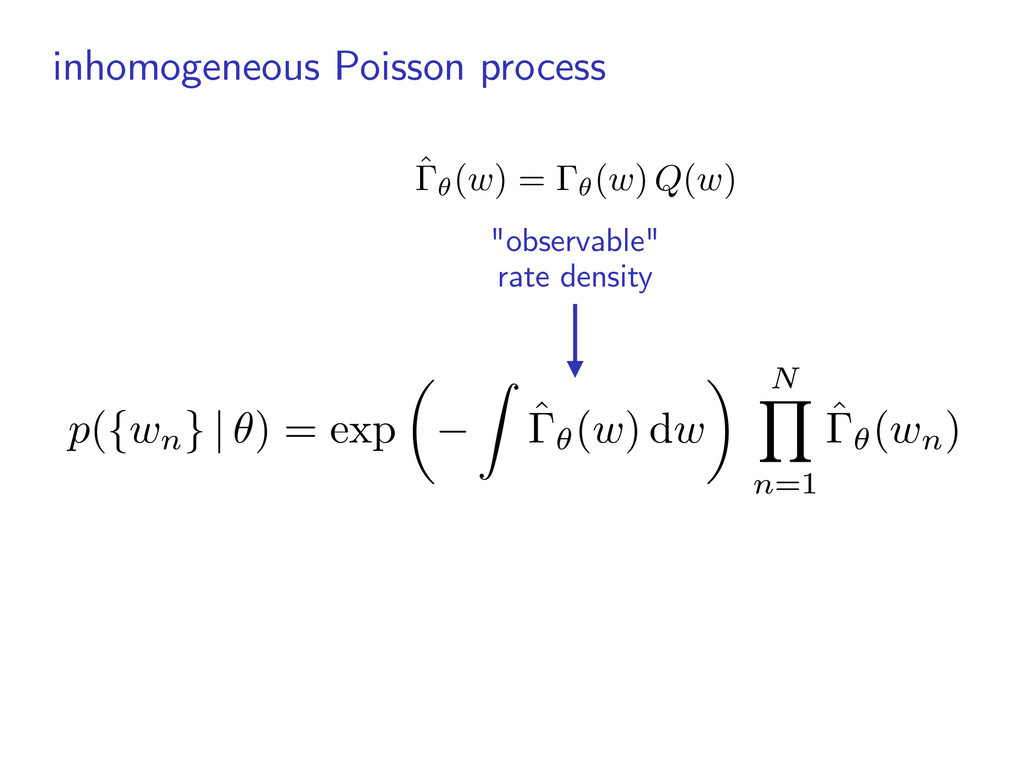
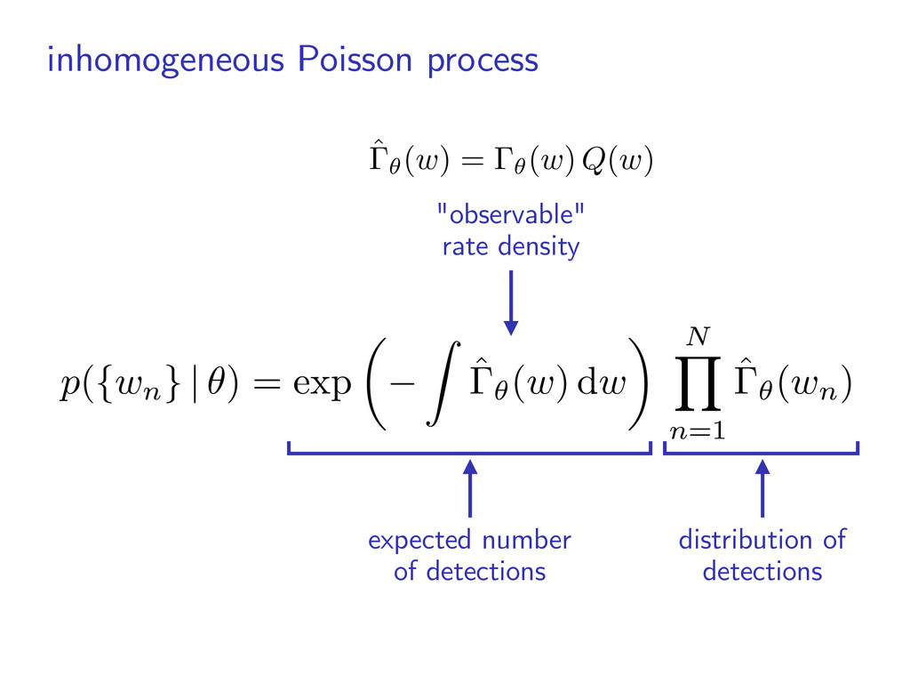
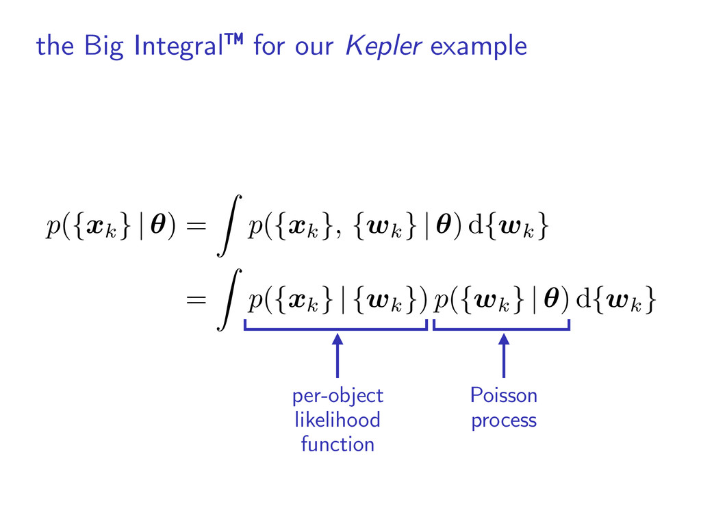
24. ▶︎ the inverse detection efficiency procedure: weighted histogram of the catalog ▶︎ the inhomogeneous Poisson process: equation for the likelihood of the catalog methods for population inference (occurrence rate calculations)
25. inhomogeneous Poisson process p ( {wn } | ✓ ) = exp ✓ Z ˆ✓( w ) d w ◆ N Y n=1 ˆ✓( wn)
26. inhomogeneous Poisson process p ( {wn } | ✓ ) = exp ✓ Z ˆ✓( w ) d w ◆ N Y n=1 ˆ✓( wn) "observable" rate density ˆ ✓(w) = ✓(w) Q(w)
27. expected number of detections inhomogeneous Poisson process p ( {wn } | ✓ ) = exp ✓ Z ˆ✓( w ) d w ◆ N Y n=1 ˆ✓( wn) "observable" rate density ˆ ✓(w) = ✓(w) Q(w)
28. distribution of detections expected number of detections inhomogeneous Poisson process p ( {wn } | ✓ ) = exp ✓ Z ˆ✓( w ) d w ◆ N Y n=1 ˆ✓( wn) "observable" rate density ˆ ✓(w) = ✓(w) Q(w)
29. observable rate density ▶︎ includes detection efficiency ▶︎ "true" rate density: histogram, power law, physical model, etc. ▶︎ can include false positives/alarms ▶︎ multiple surveys? product of likelihoods ˆ ✓(w) = ✓(w) Q(w)
30. aside: inverse detection efficiency ✓j = Nj R j Q(w) dw
31. aside: inverse detection efficiency ✓j = Nj R j Q(w) dw bin height
32. aside: inverse detection efficiency ✓j = Nj R j Q(w) dw bin height number of points in bin
33. aside: inverse detection efficiency ✓j = Nj R j Q(w) dw bin height survey completeness or detection efficiency number of points in bin
34. aside: inverse detection efficiency ✓j = Nj R j Q(w) dw bin height survey completeness or detection efficiency bin volume number of points in bin
35. aside: inverse detection efficiency ✓j = Nj R j Q(w) dw bin height survey completeness or detection efficiency bin volume number of points in bin ✓j = Nj X n=1 1 Q(wn)
36. what about uncertainties & missing data?
37. DO NOT TRY THIS AT HOME! attempt #1 — intuition
38. attempt #1: intuition DO NOT TRY THIS AT HOME! truth w p(w)
39. attempt #1: intuition DO NOT TRY THIS AT HOME! ignoring uncertainties truth w p(w)
40. attempt #1: intuition DO NOT TRY THIS AT HOME! ignoring uncertainties truth intuitive resampling w p(w)
41. attempt #1: intuition DO NOT TRY THIS AT HOME! ignoring uncertainties truth intuitive resampling w p(w) BAD IDEA
42. the moral? ▶︎ don't be caught adding your posteriors! ▶︎ use hierarchical inference instead
43. attempt #2 — hierarchical inference
44. per-object likelihood function Poisson process p({ xk } | ✓ ) = Z p({ xk }, { wk } | ✓ ) d{ wk } = Z p({ xk } | { wk }) p({ wk } | ✓ ) d{ wk } the Big Integral™ for our Kepler example
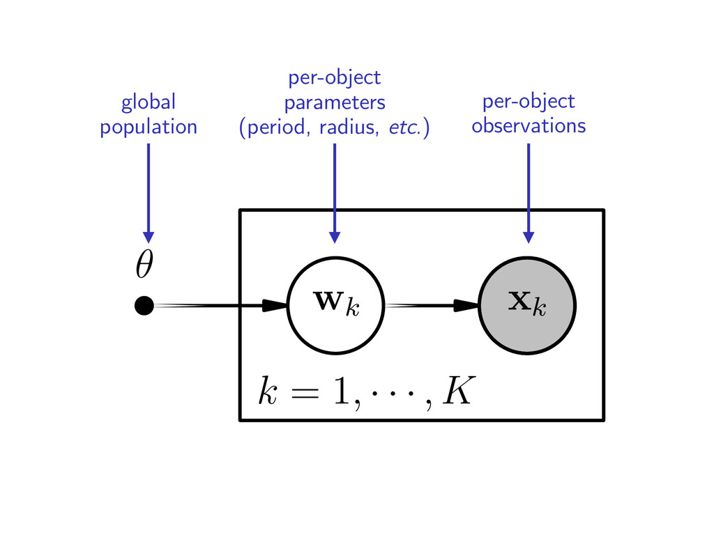
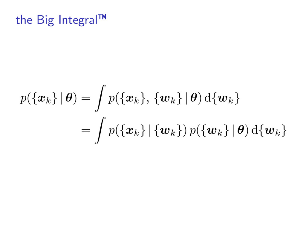
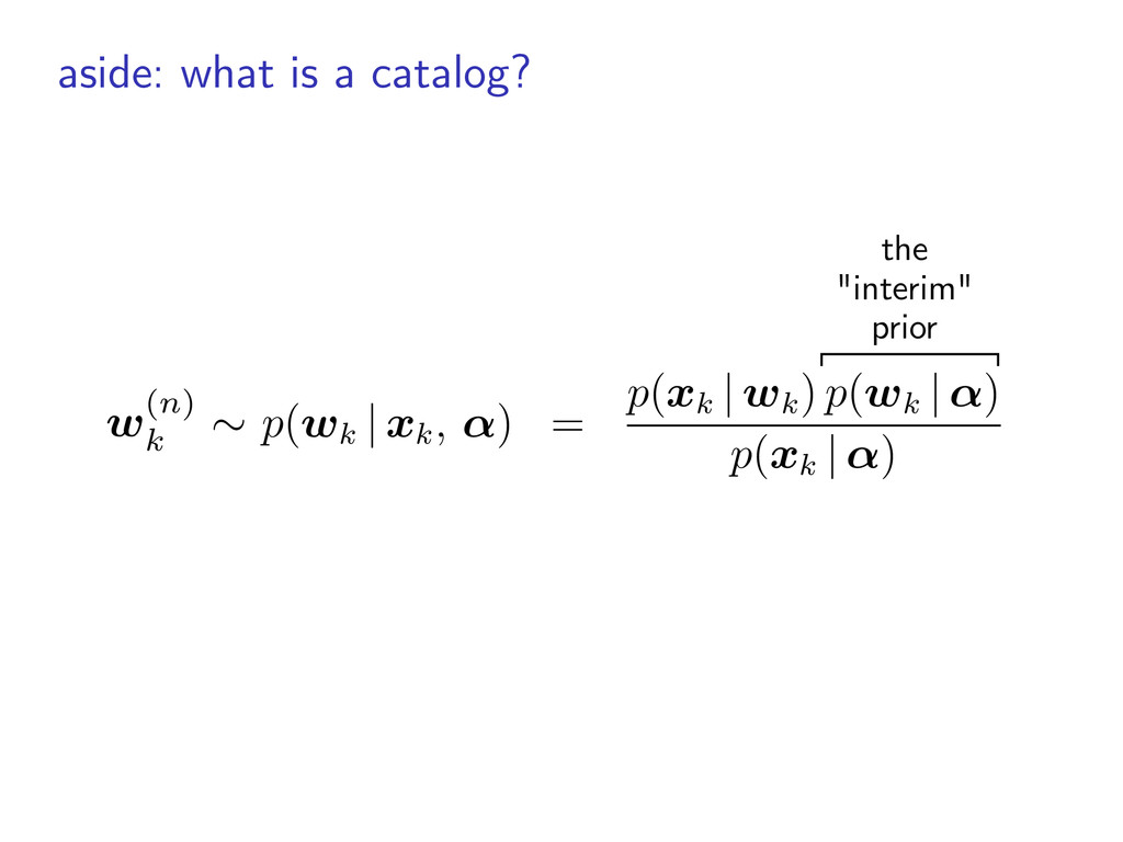
45. the "interim" prior aside: what is a catalog? w (n) k ⇠ p( wk | xk, ↵ ) – 8 – we will reuse the hard work that went into building the ca ach entry in a catalog is a representation of the posterior p p( wk | xk , ↵ ) = p( xk | wk ) p( wk | ↵ ) p( xk | ↵ ) meters wk conditioned on the observations of that object nder that the catalog was produced under a specific cho ive”— interim prior p( wk | ↵ ). This prior was chosen by the di↵erent from the likelihood p( wk | ✓ ) from Equation (2). e can use these posterior measurements to simplify Equa
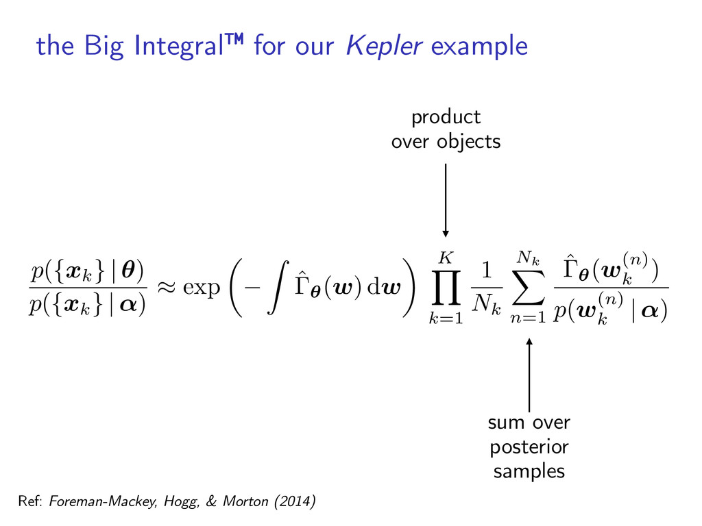
46. the Big Integral™ for our Kepler example p ( { xk } | ✓) p ( { xk } | ↵) ⇡ exp ✓ Z ˆ✓(w) dw ◆ K Y k=1 1 Nk Nk X n=1 ˆ✓(w (n) k ) p (w (n) k | ↵) sum over posterior samples product over objects Ref: Foreman-Mackey, Hogg, & Morton (2014)
47. when does all this matter? ▶︎ when you want precise measurements with realistic uncertainty estimates ▶︎ near detection limit (esp. extrapolation!) ▶︎ missing data ▶︎ ...
48. summary ▶︎ hierarchical inference and probabilistic modeling provide a consistent framework for: ▶︎ measurement uncertainties ▶︎ missing data ▶︎ heterogeneous datasets ▶︎ false positives/alarms ▶︎ ... ▶︎ it isn't always hard