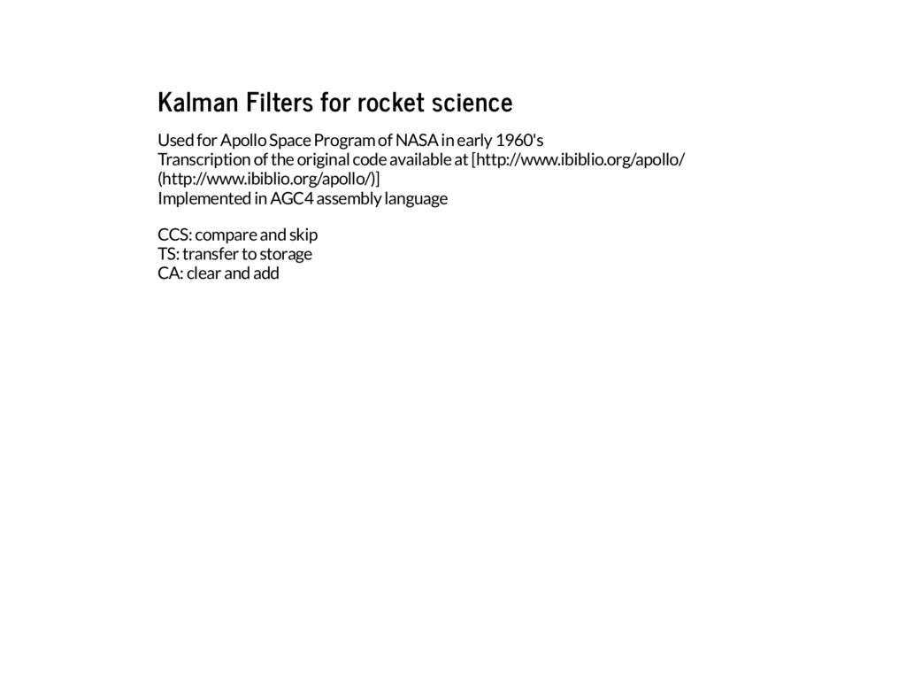
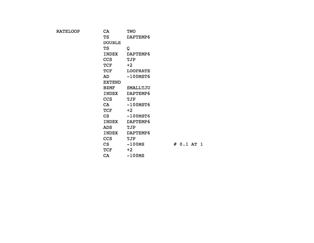
of NASA in early 1960's Transcription of the original code available at [ ] Implemented in AGC4 assembly language CCS: compare and skip TS: transfer to storage CA: clear and add http://www.ibiblio.org/apollo/ (http://www.ibiblio.org/apollo/)
= numpy.dot(A, numpy.dot(P, A.T)) + R K = numpy.dot(P, numpy.dot(A.T, numpy.linalg.inv(C))) u = u + numpy.dot(K, (b - numpy.dot(A, u))) P = P - numpy.dot(K, numpy.dot(C, K.T)) return u, P
1]]) u = numpy.zeros((2, 1)) # Random initial measurement centered at state value b = numpy.array([[u[0, 0] + randn(1)[0]], [u[1, 0] + randn(1)[0]]]) P = numpy.diag((0.01, 0.01)) F = numpy.array([[1.0, dt], [0.0, 1.0]]) # Unit variance for the sake of simplicity Q = numpy.eye(u.shape[0]) R = numpy.eye(b.shape[0])
[], [] for k in numpy.arange(0, N): u, P = predict(u, P, F, Q) predictions.append(u) u, P = correct(u, A, b, P, Q, R) corrections.append(u) measurements.append(b) b = numpy.array([[u[0, 0] + randn(1)[0]], [u[1, 0] + randn(1)[0]]]) print 'predicted final estimate: %f' % predictions[-1][0] print 'corrected final estimate: %f' % corrections[-1][0] print 'measured state: %f' % measurements[-1][0] predicted final estimate: -23.417806 corrected final estimate: -22.995292 measured state: -22.720059
![In [29]: def predict(u, P, F, Q): u = numpy.dot(F,](https://files.speakerdeck.com/presentations/0aee8fd8f93442b18375f34d9b20e31c/slide_16.jpg)
![In [30]: def correct(u, A, b, P, Q, R): C](https://files.speakerdeck.com/presentations/0aee8fd8f93442b18375f34d9b20e31c/slide_18.jpg)
![In [124]: dt = 0.1 A = numpy.array([[1, 0], [0,](https://files.speakerdeck.com/presentations/0aee8fd8f93442b18375f34d9b20e31c/slide_19.jpg)
![In [125]: N = 100 predictions, corrections, measurements = [],](https://files.speakerdeck.com/presentations/0aee8fd8f93442b18375f34d9b20e31c/slide_20.jpg)
![In [126]: t = numpy.arange(50, 100) fig = plt.figure(figsize=(15,15)) axes](https://files.speakerdeck.com/presentations/0aee8fd8f93442b18375f34d9b20e31c/slide_21.jpg)
![Thank you! [email protected] @eramirem](https://files.speakerdeck.com/presentations/0aee8fd8f93442b18375f34d9b20e31c/slide_23.jpg)