Numerical Analysis for Orbit Propagation

Transcript

1. Numerical Analysis for Orbit Propagation (in Python) Elizabeth Ramirez - er2732@columbia.edu Columbia University - Department of Applied Mathematics Pasadena, Dec 14 2016
2. Motivation Commercial and Open-Source Orbit Propagators SDK (AGI): RK4: Runge-Kutta 4th order RK7(8): Runge-Kutta 7th order, 8th order error control RKV8(9): Runge-Kutta-Verner SciPy: dopri5: explicit RK(4)5 due to Dormand & Prince dopri853: explicit RK8(5,3)
3. Part I: Numerical Methods for IVP
4. General Form
5. N-Body Problem ODE
6. In [ ]: def rhs_two_body(t, U, mu=398600.4415): """ Right-hand side 2-body problem ODE Input Parameters t <numpy.float64>: time step U <numpy.ndarray>: state vector Output Parameters f_U <numpy.ndarray>: evaluation of RHS """ r = U[0:3] v = U[3:6] dr = v dv = -mu*r/(numpy.linalg.norm(r)**3) f_U = numpy.zeros(6) f_U[0:3] = dr f_U[3:6] = dv return f_U
7. Existence and Uniqueness Is our RHS continuous? Is our RHS differentiable continuous?
8. Lipschitz Continuity Lipschitz continuity guarantee uniqueness at least up to some time T
9. Existence and Uniqueness Q: Is our RHS Lipschitz continuous? A: If f: it can be shown that it satis es Lipschitz continuity with where = maximum of all partial derivatives in our domain "Almost Everywhere"
10. Part II: Numerical Methods and Error Analysis
11. Basic Schemas Forward Euler: Backward Euler (Implicit): Leapfrog: Trapezoidal (Implicit):
12. One-step Methods: Runge-Kutta Family Compute intermediate stages to derive higher-order solvers. Only uses current evaluation. Number of stages Order of accuracy (only true for lower numbers) Ex : Runge-Kutta 2 stages. Approximate the solution at Intermediate stage: Final stage:
13. In [ ]: def ERK2(t, r, v, f): """ Explicit Runge-Kutta 2-stage Input Parameters t <numpy.ndarray>: time vector r, v <numpy.ndarray>: initial conditions f <function>: RHS function Output Parameters U <numpy.ndarray>: solution state vector """ U = numpy.zeros((6, t.shape[0])) U[0:3, 0] = r U[3:6, 0] = v delta_t = t[1] - t[0] for (n, t_n) in enumerate(t[1:]): U[:, n+1] = U[:, n] + 0.5 * delta_t * f(t_n, U[:, n]) U[:, n+1] = U[:, n] + delta_t * f(t_n, U[:, n+1]) return U
14. RK4
15. In [ ]: def ERK4(t, r, v, f): """ Explicit Runge-Kutta 4-stage """ U = numpy.zeros((6, t.shape[0])) U[0:3, 0] = r U[3:6, 0] = v delta_t = t[1] - t[0] for (n, t_n) in enumerate(t[1:]): y_1 = delta_t*f(t_n, U[:, n]) y_2 = delta_t*f(t_n + delta_t/2.0, U[:, n] + y_1/2.0) y_3 = delta_t*f(t_n + delta_t/2.0, U[:, n] + y_2/2.0) y_4 = delta_t*f(t_n + delta_t, U[:, n] + y_3) U[:, n+1] = U[:, n] + 1.0/6.0*(y_1 + 2.0*y_2 + 2.0*y_3 + y_4) return U
16. Implicit RK : zeros of the Legendre Polynomial of degree 2: : related to quadrature formula in a interval: "Gauss-Legendre methods are the Lamborghinis of the numerical ODE world. They are expensive and hard to drive, but they have style!" C.J.Budd, University of Bath (England)
17. In [ ]: def IRKGL(t, r, v, f): """ Implicit Runge-Kutta Gauss-Legendre 2-stage """ A = numpy.array(...) b = numpy.array(...) c = numpy.array(...) U = numpy.zeros((6, t.shape[0])) U[0:3, 0] = r U[3:6, 0] = v delta_t = t[1] - t[0] for i in xrange(t.shape[0] - 1): # Set stage function evaluations y1=0 and y2=0 K = numpy.zeros((6, 2)) D = numpy.dot(K, A.T) # a_11*u1 + a_12*u2 # Initial guess for k1 and k2 K_new = numpy.zeros((6, 2)) K_new[:, 0] = f(t + c[0]*delta_t, U[:,i] + delta_t*D[:, 0]) K_new[:, 1] = f(t + c[1]*delta_t, U[:,i] + delta_t*D[:, 1]) # Solve nonlinear system for stage evaluations error = numpy.max(numpy.abs(K - K_new)) tolerance = 1e-08 while error > tolerance: K = K_new.copy() D = numpy.dot(K, A.T) K_new[:, 0] = f(t + c[0]*delta_t, U[:,i] + delta_t*D[:, 0]) K_new[:, 1] = f(t + c[1]*delta_t, U[:,i] + delta_t*D[:, 1]) error = numpy.max(numpy.abs(K - K_new)) U[:, i+1] = U[:, i] + delta_t*numpy.dot(K_new, b).reshape(6) return U
18. Linear Multistep Methods If , the method is explicit. In practice, we normally use .
19. Adams Methods
20. Adams-Bashforth Explicit Methods Pick up to eliminate as many terms of the truncation error as possible Requires bootstrapping 2-step: 4-step:
21. Adams-Moulton Implicit Methods One order of accuracy greater 2-step :
22. In [ ]: def ABM3(t, r, v, f): """ Adams-Bashforth-Moulton 3-step Predictor-Corrector """ U = numpy.empty((6, t.shape[0])) U[:, :3] = ERK4(t[0:3], r, v, f) # Bootstrap with RK4 delta_t = t[1] - t[0] for n in xrange(t.shape[0] - 3): U[:, n+3] = U[:, n+2] + (delta_t/12.0)*(5.0*f(t[n], U[:, n]) - 16.0*f(t[n+1], U[:, n+1]) + 23.0*f(t[n+2], U[:, n+2])) U[:, n+3] = U[:, n+2] + delta_t/24.0*(f(t[n], U[:, n]) - 5.0*f(t[n+1], U[:, n+1]) + 19.0*f(t[n+2], U[:, n+2]) + 9.0*f(t[n+3], U[:, n+3])) return U
23. Error Analysis Truncation Error: Method is consistent if Order of accuracy Assume approximation to be of the form: p-order accurate: Model error as: where is order of accuracy
24. Truncation Error Forward Euler Centered Approximation RK2
25. Truncation Error LMM Consistent only if terms in the expansion of with vanish, thus, and
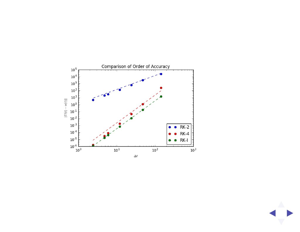
26. In [ ]: """ Visualization of Order of Accuracy """ # In general, we expect error to behave as this C = lambda delta_x, error, order: error / delta_x**order # Use RHS for 2-body problem f = rhs_two_body # Initial conditions r = [5492.000, 3984.001, 2.955] v = [-3.931, 5.498, 3.665] # Gravitational constant for Earth mu = 398600.4415 # Final time for simulation t_f = 86400 # From coarser to finer grid steps = [600, 1800, 3600, 7200, 14400, 18000, 36000] # Calculate errors for distance vector; we want quantities to be # comparable. Use matrix norm with ord=1 (max sum along axis 0) error_rk2[i] = numpy.linalg.norm((U_RK2[0:3, :] - U[0:3, :]), ord=1) # Plot expected order of accuracy axes.loglog(delta_t, C(delta_t[1], error_rk2[1], 2.0) * delta_t**2.0, '--b') axes.loglog(delta_t, C(delta_t[1], error_rk4[1], 4.0) * delta_t**4.0, '--r') axes.loglog(delta_t, C(delta_t[1], error_irk[1], 4.0) * delta_t**4.0, '--g')
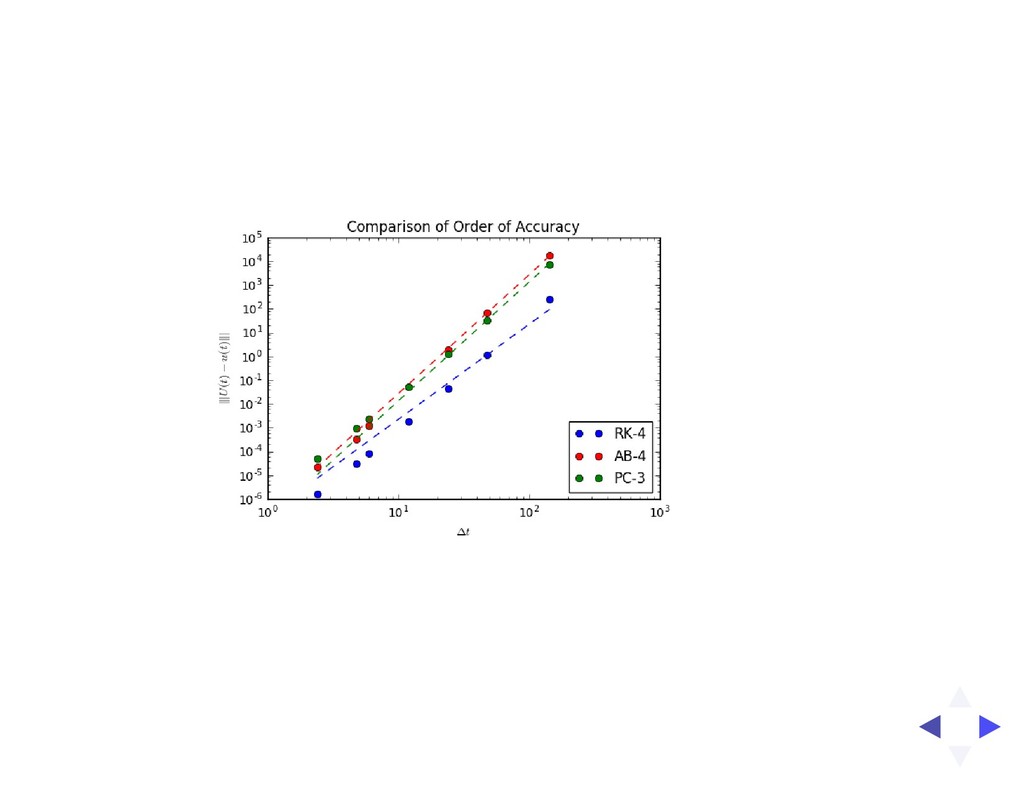
28. In [ ]: axes.loglog(delta_t, order_C(delta_t[1], error_rk[1], 4.0) * delta_t**4.0, '--b') axes.loglog(delta_t, order_C(delta_t[1], error_ab[1], 5.0) * delta_t**5.0, '--r') axes.loglog(delta_t, order_C(delta_t[1], error_pc[1], 5.0) * delta_t**5.0, '--g')
30. Part III: Convergence and Stability
31. Convergence Recall our ODE general form: We want: : nal time : number of steps
32. Convergence For our method to be convergent we require that it is: consistent: zero-stable: sum of total errors as is bounded and has the same order as truncation error
33. General one-step method convergence Forward Euler Expanding back to time tn=0 We want to bound
34. Zero-stability for LMM Even if the coef cients satisfy the consistency condition, the global error of the method might not converge. Characteristic Polynomial : solve ODE using our LMM An r-step LMM is zero-stable if the roots of satisfy the conditions: for are not repeated. If there are repeated they must be
35. Characteristic Polynomial of Adams Methods General form: Roots of this polynomial are: All Adams Methods are zero-convergent, and since they satisfy the consistence condition, all Adams LMM are convergent.
36. Stability regions What we want: within the stability region, including large eigenvalues No LMM is A-stable Non-linear problem: Find such that is within the stability region, where are the eigenvalues of Jacobian matrix Implicit methods have half-plane stability regions or better For stiff problems, we expect: the more accurate, the "smaller" the stability region.
37. A-stability Find eigenvalues for nonlinear system:
40. Conclusions Both Gauss-Legendre implicit method and Runge-Kutta fourth-order method showed very good results in terms of accuracy The Gauss Legendre method proved to be much more stable (implicit methods are) than the explicit Runge-Kutta when increasing the time step. However, is much more dif cult to program since it requires initial guesses and extra iterations that carry extra evaluations of the righ-hand side function, requiring more computational time. A balance between accuracy, stability and computational resources is desirable For explicit methods, instability leads to loss of information. LMM are consistend and zero-stable but unstable computations can appear if problem is very stiff.
41. Conclusions Fortran arrays are much better than NumPy’s Fewer lines of code with Python In the future: Maybe Julia? Switch to PyPy's fork of Numpy, NumPyPy? most functionality has been already ported. (JIT compiler)
42. Thank you!