Upgrade to Pro — share decks privately, control downloads, hide ads and more …

Business Intelligence - Tecnologias para auxili...

Business Intelligence - Tecnologias para auxiliar na tomada de decisões

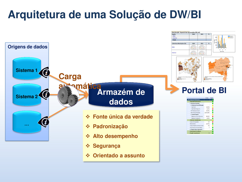
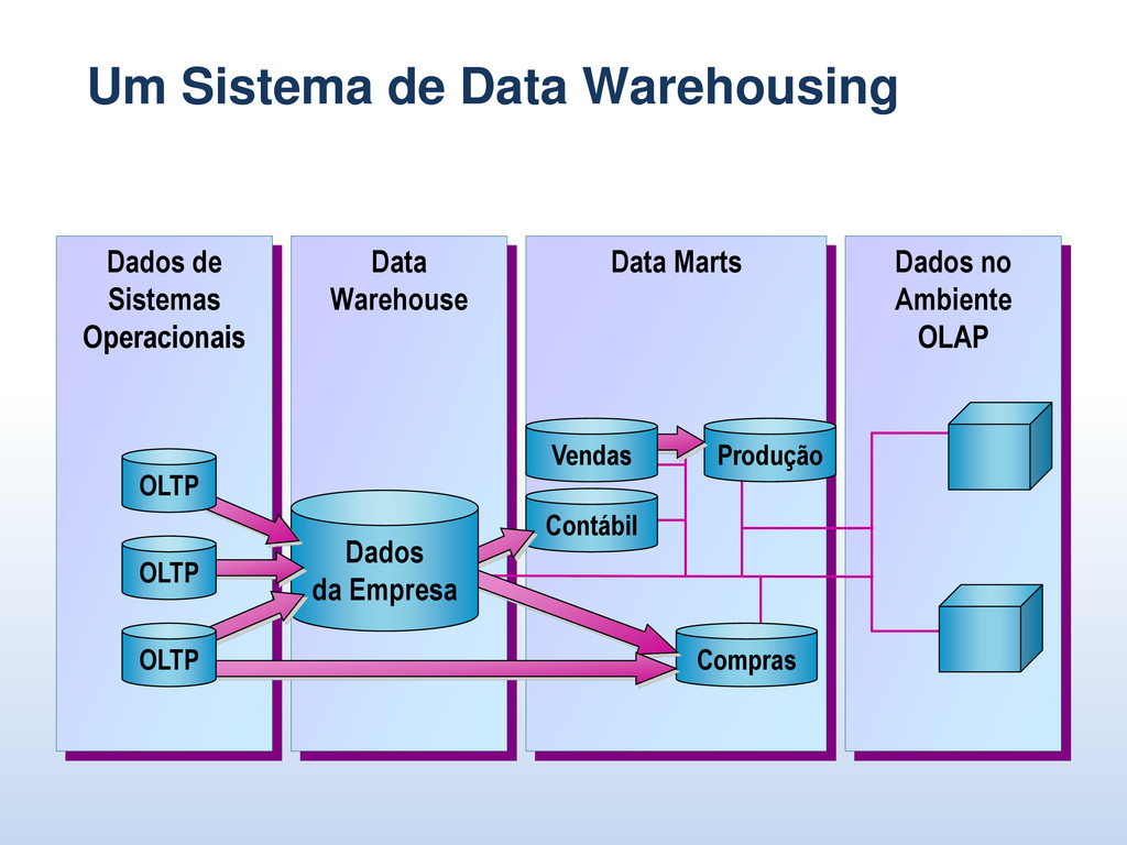
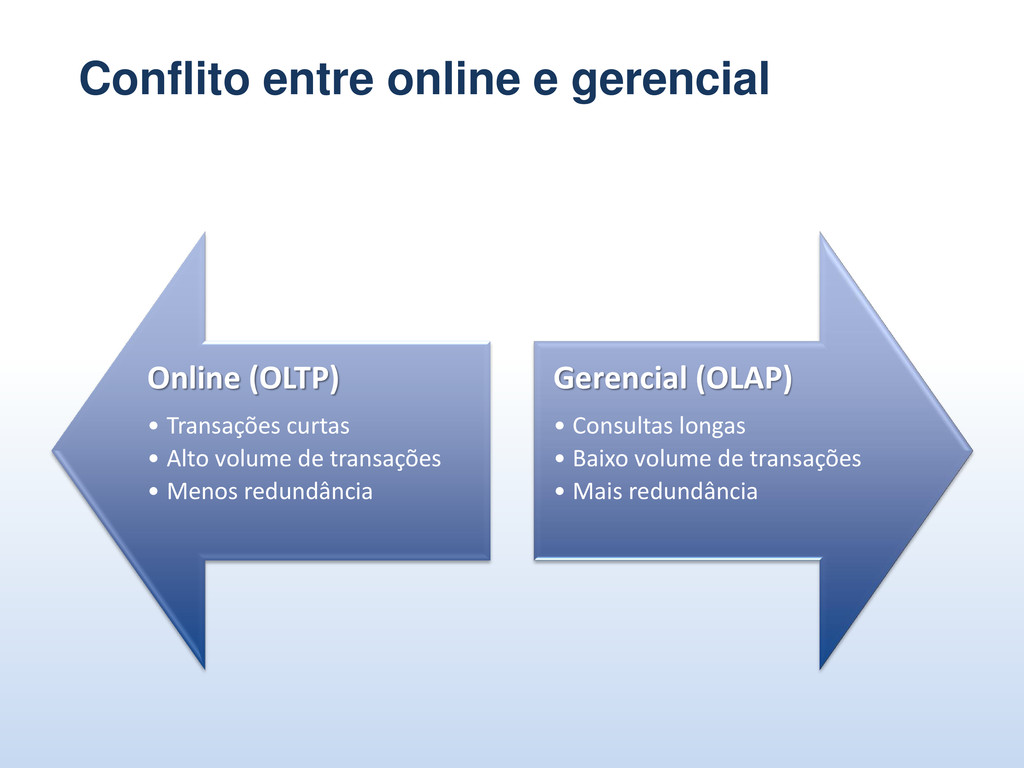
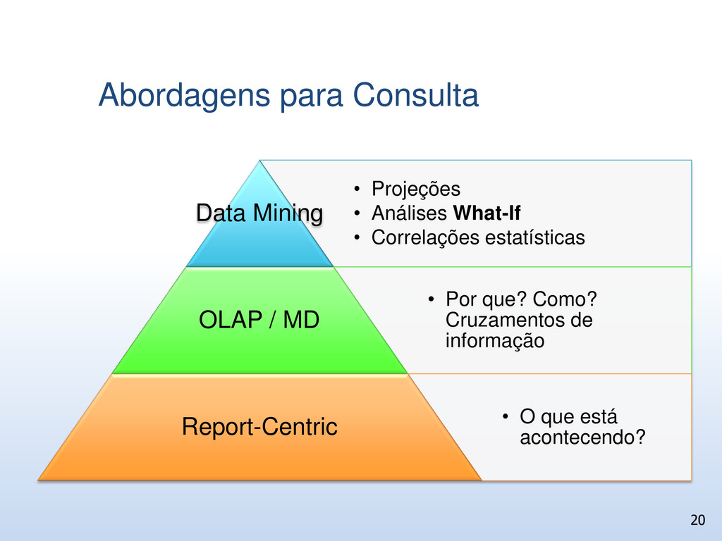
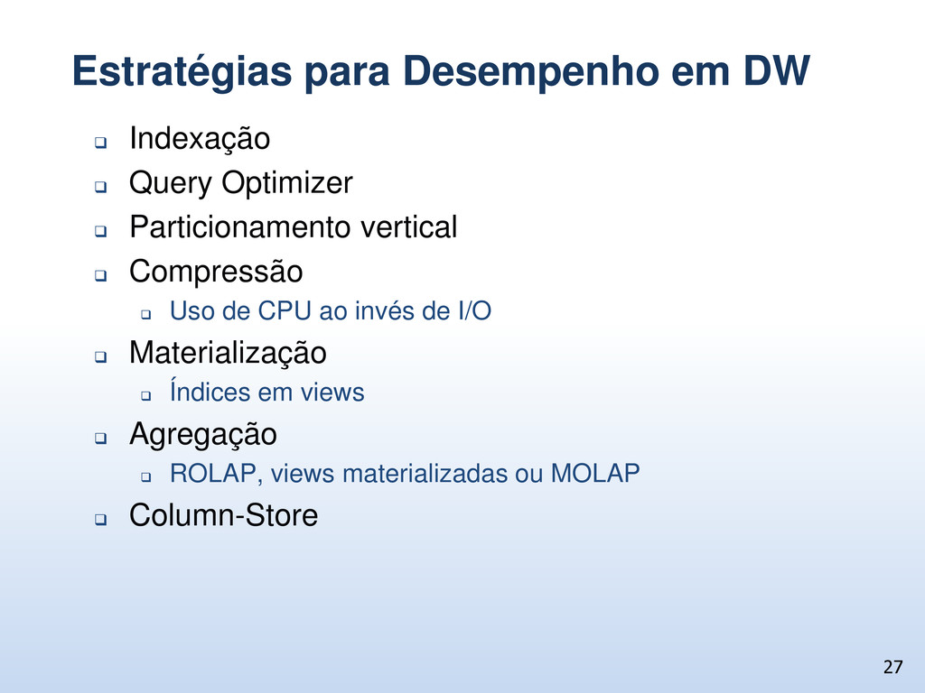
Conheça um pouco mais sobre as tecnologias de Business Intelligence que auxiliam na tomada de decisões estratégicas. Falaremos e demonstraremos dashboards com elementos dinâmicos, consolidação de dados, Data Mining e estratégias para obter um melhor desempenho em consultas.

Avatar for Fábio Ávila

Fábio Ávila

October 30, 2012
Tweet

More Decks by Fábio Ávila

Other Decks in Technology

Transcript

  1. Fábio Ávila? Quem é esse cara?  Mestre em Ciência

    da Computação – CIn/UFPE  Benchmarks em Bancos de Dados  Diretor Presidente da Ávila Soluções  13 anos de mercado  Área de atuação: bancos de dados Microsoft, BI, portais e desenvolvimento de software  Microsoft Gold Partner: Business Intelligence e Data Platform  Técnico Empresário 2
  2. Time travel back to 1980  Dominate hardware platform was

    the Digital VAX 11/780  1 MIPS CPU w. 1KB of cache memory  8 MB memory (maximum)  80 MB disk drives w. 1 MB/second transfer rate  $250K purchase price!  INGRES & Oracle were the dominant vendors  Same basic DBMS architecture as is in use today 3 Query engine Buffer pool
  3.  Basic RDMS design is essentially unchanged  Except for

    scale-out using parallelism  But the hardware landscape has changed dramatically: Since 1980 Today 4 RDBMS CPU CPU Caches Memory Disks 1980 1 MIPS 1 KB 2 MB/CPU 80 MB Today CPU Caches CPU Memory Disks 2 GIPS 1 MB 2 GB/CPU 800 GB 2,000X 1,000X 1,000X 10,000X
  4. A little closer look at 30 year disk trends Capacities:

    80 MB  800 GB - 10,000X Transfer rates: 1.2 MB/sec  80 MB/sec - 65X Avg. seek times: 30 ms  3 ms - 10X (30 I/Os/sec  300 I/Os/sec) The significant differences in these trends (10,000X vs. 65X vs. 10X) have had a huge impact on both OLTP and data warehouse workloads (as we will see) 5
  5. 1980 1985 1975 Looking at OLTP  Consider TPC A/B

    results from 1985:  Fastest system was IBM’s IMS Fastpath DBMS running on a top-of-the-line IBM 370 mainframe at 100 TPS with 4 disk I/Os per transaction:  100 TPS  400 disk I/Os/second  @ 30 I/Os/sec. per drive 14 drives  Fastest relational products could only do 10 TPS 6
  6. 2020 2030 2009  After 30 years of CPU and

    memory improvements, SQL Server on a modest Intel box can easily achieve 25,000 TPS (TPC-B)  25,000 TPS  100,000 disk I/Os/second  @300 I/Os/sec per drive  330 drives!!!  Relative performance of CPUs and disks is totally out of whack 8
  7. OLTP Takeaway  The benefits from a 1,000x improvement in

    CPU performance and memory sizes are almost negated by the 10X in disk accesses/second  Forcing us to run our OLTP systems with 1000s of mostly empty disk drives  No easy software fix, unfortunately  SSDs provide the only real hope 9
  8. Turning to Data Warehousing  Two key hardware trends have

    had a huge impact on the performance of single box relational DB systems:  The imbalance between disk capacities and transfer rates  The ever increasing gap between CPU performance and main memory bandwidth 10
  9. Looking at Disk Improvements  Incredibly inexpensive drives (& processors)

    have made it possible to collect, store, and analyze huge quantities of data 11 But, consider the metric transfer bandwidth/byte Over the last 30 years Capacity: 80MB  800GB 10,000x Transfer Rates: 1.2MB/sec  80MB/sec 65x  1980: 1.2 MB/sec / 80 MB = 0.015  2009: 80 MB/sec / 800,000 MB =.0001 When relative capacities are factored in, drives are 150X slower today!!!
  10. Another Viewpoint  1980  30 random I/Os/sec @ 8KB

    pages  240KB/sec  Sequential transfers ran at 1.2 MB/sec  Sequential/Random 5:1  2009  300 random I/Os/sec @ 8KB pages  2.4 MB/sec  Sequential transfers run at 80 MB/sec  Sequential/Random 33:1  Takeaway: DBMS must avoid doing random disk I/Os whenever possible 12
  11. Data Warehouse “Coleção de dados orientada a assunto, integrada, não-volátil

    e variante no tempo, utilizada para tomada de decisões”. - W. H. Inmon “Uma cópia de dados transacionais estruturada especificamente para consulta e análise" R. Kimball
  12. Data Warehouse “Repositório estruturado e corporativo de dados orientados a

    assunto, variantes no tempo e históricos, usados para recuperação de informações e suporte à decisão. O DW armazena dados atômicos e sumarizados”. - Definição de DW da Oracle
  13. Origens de dados Arquitetura de uma Solução de DW/BI Sistema

    1 Sistema 2 … Armazém de dados Portal de BI  Fonte única da verdade  Padronização  Alto desempenho  Segurança  Orientado a assunto Carga automática
  14. Um Sistema de Data Warehousing Dados no Ambiente OLAP Data

    Marts Data Warehouse Dados de Sistemas Operacionais Compras Produção Contábil Dados da Empresa OLTP OLTP OLTP Vendas
  15. Conflito entre online e gerencial Online (OLTP) • Transações curtas

    • Alto volume de transações • Menos redundância Gerencial (OLAP) • Consultas longas • Baixo volume de transações • Mais redundância
  16. Abordagens para Consulta 20 • Projeções • Análises What-If •

    Correlações estatísticas Data Mining • Por que? Como? Cruzamentos de informação OLAP / MD • O que está acontecendo? Report-Centric
  17. Soluções de Relatórios  Report-Centric  TI entrega a estrutura

    do relatório com filtros  Servidor de relatórios + designer  Componentes dinâmicos  Interactive Visualization Tools  Cubos  Modelos In-Memory (ex: BISM)  Data Mining 21
  18. Demo – Abordagens para Consulta  Report-Centric  SQL Server

    Reporting Services  Filtros do MS Pivot  BISM  Power View  Data Mining  Data Mining AddIn for Excel  Navegação  Tabela dinâmica: drill-up, drill-down, drill-through, slice, dice 23
  19. Critérios de Inclusão • $15 milhões anuais de licença (2011)

    • 9 de 13 capacidades (2011) – (1) Estrutura de BI, (2) Gerenciamento de metadados – (3) Ferramentas de desenvolvimento, (4) Colaboração – (5) Relatórios, (6) Dashboards, (7) Consulta ad hoc – (8) Integração com o MS Office – (9) BI baseado em busca, (10) OLAP – (11) Visualização interativa – (12) Data mining, (13) Scorecards • 1.364 questionários de clientes (2012)
  20. Eixos • Habilidade de execução – Competitividade, recursos, qualidade –

    Continuidade, saúde financeira, plano de investimentos do fabricante – Licenciamento, pré-venda, negociação – Habilidade para adaptar a mudanças de mercado / capacidade de marketing e divulgação – Suporte ao produto pelo fabricante. • Completude de visão – Roadmap, Inovação e Marketing – Habilidade de entender a necessidade dos usuários – Comunicação do valor e diferenciação ao mercado – Combinação de recursos para estender seu mercado – Adequação para diversos setores: automobilístico, financeiro, varejo, etc. – Atender a necessidades de outros países, direta ou indiretamente
  21. Estratégias para Desempenho em DW  Indexação  Query Optimizer

     Particionamento vertical  Compressão  Uso de CPU ao invés de I/O  Materialização  Índices em views  Agregação  ROLAP, views materializadas ou MOLAP  Column-Store 27
  22. O papel do Query Optimizer (a 40.000 metros) Query Optimizer

    Comando SQL Query Plan fantástico Magic Happens
  23. What’s the Magic? Select o_year, sum(case when nation = 'BRAZIL'

    then volume else 0 end) / sum(volume) from ( select YEAR(O_ORDERDATE) as o_year, L_EXTENDEDPRICE * (1 - L_DISCOUNT) as volume, n2.N_NAME as nation from PART, SUPPLIER, LINEITEM, ORDERS, CUSTOMER, NATION n1, NATION n2, REGION where P_PARTKEY = L_PARTKEY and S_SUPPKEY = L_SUPPKEY and L_ORDERKEY = O_ORDERKEY and O_CUSTKEY = C_CUSTKEY and C_NATIONKEY = n1.N_NATIONKEY and n1.N_REGIONKEY = R_REGIONKEY and R_NAME = 'AMERICA‘ and S_NATIONKEY = n2.N_NATIONKEY and O_ORDERDATE between '1995-01-01' and '1996-12-31' and P_TYPE = 'ECONOMY ANODIZED STEEL' and S_ACCTBAL <= constant-1 and L_EXTENDEDPRICE <= constant-2 ) as all_nations group by o_year order by o_year Consider Query 8 of the TPC-H benchmark: Plan 1 Plan 2 Plan 3 Plan 4 Plan 5 … There about 22 million alternative ways of executing this query! A very big haystack to be searching through The QO must select a plan that runs in seconds or minutes, not days or weeks! Should not take hours or days to pick a plan!
  24. A First Example 30 Query Execution Engine Query Optimizer Parser

    SELECT Average(Rating) FROM Reviews WHERE MID = 932 Reviews Date CID MID Rating … … … … Logical operator tree Avg (Rating) Select MID = 932 Reviews Query Plan #1 Avg_agg [Cnt, Sum] Scan Reviews Filter MID = 932 Avg_agg [Cnt, Sum] Index Lookup MID = 932 MID Index Reviews Query Plan #2 or
  25. Customers table – one file/attribute id 1 2 3 4

    5 6 7 8 9 Tables are stored “column-wise” with all values from a single column stored in a single file “Column Store” Table Layout 31 Customers table – user’s view id Name Address City State BalDue 1 Bob … … … $3,000 2 Sue … … … $500 3 Ann … … … $1,700 4 Jim … … … $1,500 5 Liz … … … $0 6 Dave … … … $9,000 7 Sue … … … $1,010 8 Bob … … … $50 9 Jim … … … $1,300 BalDue $3,000 $500 $1,700 $1,500 $0 $9,000 $1,010 $50 $1,300 State … … … … … … … … … City … … … … … … … … … Address … … … … … … … … … Name Bob Sue Anne Jim Liz Dave Sue Bob Jim
  26. A Concrete Example Assume:  Customer table has 10M rows,

    200 bytes/row (2GB total size)  Id and BalDue values are each 4 bytes long, Name is 20 bytes Query: Select id, Name, BalDue from Customer where BalDue > $1000 Row store execution Scan 10M rows (2GB) @ 80MB/sec = 25 sec. Column store execution Scan 3 columns, each with 10M entries 280MB@80MB/sec = 3.5 sec. (id 40MB, Name 200MB, BalDue 40MB) About a 7X performance improvement for this query!! But we can do even better using compression 32
  27. Demo – PowerPivot for Excel  Evolução da tabela dinâmica

     Column-Store no Excel  Download gratuito, compatível apenas para Excel 2010  DAX: nova linguagem para facilitar consultas  Exemplo: NBA 33