FISH 6003: Week 2 - Data Exploration

FISH 6003 Week 2

Transcript

1. Chapter 2: Data Exploration CatchRate ~ Poisson (μ ij ) E(CatchRate) = μ ij Log(μ ij ) = GearType ij + Temperature ij + FleetDeployment i FleetDeployment i ~ N(0, σ2) Using lme4: m <- glmer(CatchRate ~ GearType + Temperature + (1 | FleetDeployment), family = poisson) FISH 6003 FISH 6003: Statistics and Study Design for Fisheries Brett Favaro 2017 This work is licensed under a Creative Commons Attribution 4.0 International License
2. Land Acknowledgment We would like to respectfully acknowledge the territory in which we gather as the ancestral homelands of the Beothuk, and the island of Newfoundland as the ancestral homelands of the Mi’kmaq and Beothuk. We would also like to recognize the Inuit of Nunatsiavut and NunatuKavut and the Innu of Nitassinan, and their ancestors, as the original people of Labrador. We strive for respectful partnerships with all the peoples of this province as we search for collective healing and true reconciliation and honour this beautiful land together. http://www.mun.ca/aboriginal_affairs/
3. This week: • Before your analysis: Data Exploration • Performing a data exploration
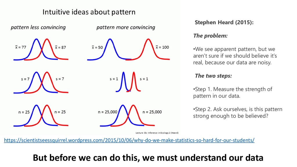
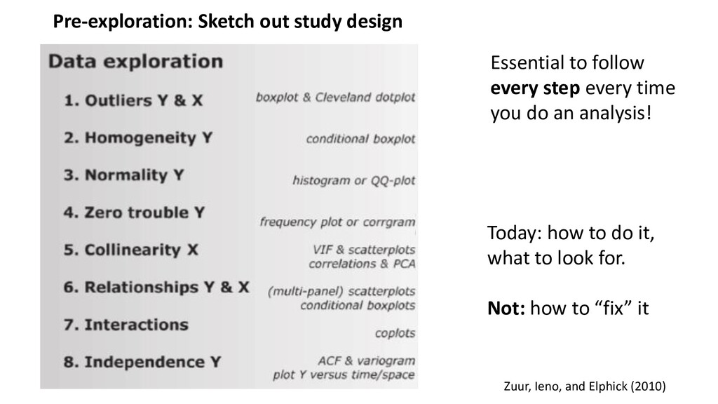
4. https://scientistseessquirrel.wordpress.com/2015/10/06/why-do-we-make-statistics-so-hard-for-our-students/ Stephen Heard (2015): The problem: •We see apparent pattern, but we aren’t sure if we should believe it’s real, because our data are noisy. The two steps: •Step 1. Measure the strength of pattern in our data. •Step 2. Ask ourselves, is this pattern strong enough to be believed? But before we can do this, we must understand our data
5. Weissgerber et al., 2015 http://journals.plos.org/plosbiology/article?id=10.1371/journal.pbio.1002128&utm_source=web&utm_medium=pdf&utm_ campaign=ppu15 Before we can apply statistical models, we need to understand what we have collected
6. Weissgerber et al., 2015 http://journals.plos.org/plosbiology/article?id=10.1371/journal.pbio.1002128&utm_source=web&utm_medium=pdf&utm_ campaign=ppu15 Before we can apply statistical models, we need to understand what we have collected
7. Weissgerber et al., 2015 http://journals.plos.org/plosbiology/article?id=10.1371/journal.pbio.1002128&utm_source=web&utm_medium=pdf&utm_ campaign=ppu15 Before we can apply statistical models, we need to understand what we have collected
8. Weissgerber et al., 2015 http://journals.plos.org/plosbiology/article?id=10.1371/journal.pbio.1002128&utm_source=web&utm_medium=pdf&utm_ campaign=ppu15 Before we can apply statistical models, we need to understand what we have collected
9. Weissgerber et al., 2015 http://journals.plos.org/plosbiology/article?id=10.1371/journal.pbio.1002128&utm_source=web&utm_medium=pdf&utm_ campaign=ppu15 Before we can apply statistical models, we need to understand what we have collected
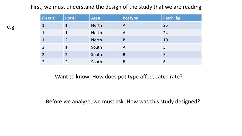
10. First, we must understand the design of the study that we are reading e.g. FleetID PotID Area PotType Catch_kg 1 1 North A 25 1 1 North A 24 1 2 North B 10 2 1 South A 5 2 2 South B 5 2 2 South B 6 Before we analyze, we must ask: How was this study designed? Want to know: How does pot type affect catch rate?
11. Was it… Or… Or… Or…
12. Was it… Area 1 Area 2 Or… Area 1 Area 2
13. Or even… Area 1 Area 2 In area 1: In area 2: What is causing difference in catch rate? Pot type, or area?
14. • We need to understand the study. Why? • Basic experimental design: • For an experiment to work, you must hold as many variables as possible constant, and change only variables of interest • e.g. don’t change pot type, location, bait, haphazardly because you can’t tell WHICH of those caused change in catch rate • If design was bad enough, you may stop right here • Could be no inference is possible • Statistically: • Because all statistical models operate on ASSUMPTIONS • Violate the assumption → Model gives you the wrong answer • False positive or false negative possible
15. 1. Design a pilot study • State hypotheses, consider statistical treatment of data 2. Do the pilot study • Analyze pilot data. Revise plans 3. Conduct power analysis 4. Do the full study 5. Explore data 6. Analyze data, report results  Today
16. http://onlinelibrary.wiley.com/doi/10.1111/j.2041-210X.2009.00001.x/full
17. Zuur, Ieno, and Elphick (2010) Essential to follow every step every time you do an analysis! Pre-exploration: Sketch out study design Today: how to do it, what to look for. Not: how to “fix” it
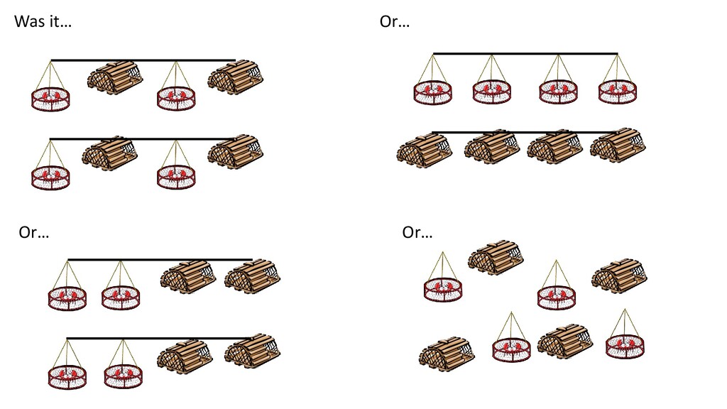
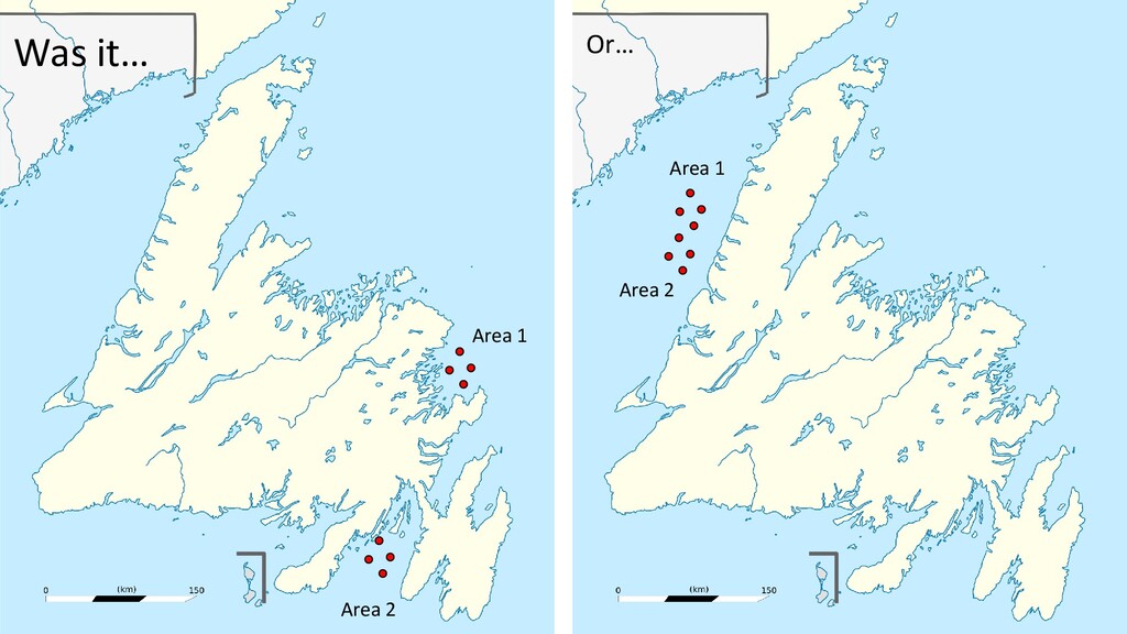
18. Pre-exploration: Study sketch • Visualize the study design • Who collected the data? • How was it grouped? • How many samples were taken/will be taken per group? • Any spatial or temporal issues? • i.e. one study, or several? One site, or several?
19. e.g. Favaro et al., 2013 https://academic.oup.com/icesjms/article/70/1/114/660896 Y: Catch per trap (# prawns) Y: Bycatch per trap (# rockfish)
20. Field test Between June and August 2010, we field-tested five BRDs (i.e. two entrance-ring and three bent-tunnel variants) as well as unmodified traps (control) to identify the BRD design that offers the best trade-off between minimizing bycatch while maintaining prawn catch. From a 9.8 m-long research vessel, we deployed gears in “strings” which contained 10 traps connected to a single line weighted with one cinder block at each end. We deployed a total of 154 strings (i.e. 1540 traps). The most common configuration of traps in each string was: two control traps (7.6 cm entrances), one trap with 7.0 cm entrances, one trap with 6.4 cm entrances, and two of each BRD variant (4-ring, 5-ring, and 7-ring), with the order of traps being randomized within each string.
21. Field test Between June and August 2010, we field-tested five BRDs (i.e. two entrance-ring and three bent-tunnel variants) as well as unmodified traps (control) to identify the BRD design that offers the best trade-off between minimizing bycatch while maintaining prawn catch. From a 9.8 m-long research vessel, we deployed gears in “strings” which contained 10 traps connected to a single line weighted with one cinder block at each end. We deployed a total of 154 strings (i.e. 1540 traps). The most common configuration of traps in each string was: two control traps (7.6 cm entrances), one trap with 7.0 cm entrances, one trap with 6.4 cm entrances, and two of each BRD variant (4-ring, 5-ring, and 7-ring), with the order of traps being randomized within each string. Tunnel Size ctrl One boat X10 / string Not all were identical? Ctrl Ctrl 7cm 6.4cm 4R 4R 5R 5R 7R 7R (order randomized)
22. Early in the study, we included PVC variants of the BRDs (so that each string had one steel and one PVC variant of each BRD type) but all PVC variants were eventually discarded because they were not durable (total of 155 PVC-BRD traps excluded). In addition, we included the 6.4 cm variant one week into the study, when we became curious about a more extreme reduction in trap opening size. One string of gear was lost during the study, while another was carried several kilometres from its original deployment site, and so its data were discarded. Three traps also became detached from one string line and were lost. Data from 1362 traps were therefore included in the present analysis (322 control traps (i.e. 7.6 cm entrances), 256 traps with 7.0 cm entrances, 145 traps with 6.4 cm entrances, 214 traps with 4-ring tunnels, 214 traps with 5- ring tunnels, and 211 traps with 7-ring tunnels). We deployed gear in two regions of southern British Columbia (Figure S1): Howe Sound, near Vancouver (49 25′ 30′′N 123820′ 00′′W), and the southern Gulf Islands, near Sidney (48 39′ 00′′N 123823′ 00′′W).
23. Early in the study, we included PVC variants of the BRDs (so that each string had one steel and one PVC variant of each BRD type) but all PVC variants were eventually discarded because they were not durable (total of 155 PVC-BRD traps excluded). In addition, we included the 6.4 cm variant one week into the study, when we became curious about a more extreme reduction in trap opening size. One string of gear was lost during the study, while another was carried several kilometres from its original deployment site, and so its data were discarded. Three traps also became detached from one string line and were lost. Data from 1362 traps were therefore included in the present analysis (322 control traps (i.e. 7.6 cm entrances), 256 traps with 7.0 cm entrances, 145 traps with 6.4 cm entrances, 214 traps with 4-ring tunnels, 214 traps with 5- ring tunnels, and 211 traps with 7-ring tunnels). Design was unbalanced Replicates We deployed gear in two regions of southern British Columbia (Figure S1): Howe Sound, near Vancouver (49 25′ 30′′N 123820′ 00′′W), and the southern Gulf Islands, near Sidney (48 39′ 00′′N 123823′ 00′′W). Two sites, far apart
24. Tunnel Size ctrl Ctrl Ctrl 7cm 6.4cm 4R 4R 5R 5R 7R 7R (order randomized) “Family” of modifications (2) Specific modifications (6) Traps are nested within strings Individual animals (if relevant) are nested within traps The design is not perfectly balanced Sites (2)
25. https://github.com/allisonhorst/stats-illustrations Know what you are measuring
27. http://onlinelibrary.wiley.com/doi/10.1111/j.2041-210X.2010.00021.x/abstract Know what you are measuring - Continuous (any #) - Count (0 to some number) - Binomial (0 or 1) - Proportion (A/B = between 0 and 1) - Nominal (unordered categories) - Ordinal (ordered categories – Likert scale) - Other (Rate?)
28. Do you know what your independent (X) variables are? • Watch for: • Is there uncertainty around X values? If yes… may be trouble! • Did you measure across the range of X values, or are there large gaps? If yes… may be trouble • In the above study: • Trap type is fixed. We know exactly what type of trap we’re fishing. Zero uncertainty. • What about environmental variables, e.g. depth? • Is there uncertainty in X? • Common problems in fisheries: • If age is on X: have you measured age correctly? How certain are you? • Putting too many decimals on X. Can you really measure to 0.01 cm? Or should you bin to nearest integer?
29. Independence of replicates is core assumption in many models Are observations independent? “Pseudoreplication is defined as the use of inferential statistics to test for treatment effects with data from experiments where either treatments are not replicated (though samples may be) or replicates are not statistically independent.” Independence = Y value at Xi is not influenced by other Xi values
30. Good fishing site Y: Catch per trap Traps are nested within strings. They are likely not independent: I.e. traps within a string are likely to be more similar to each other than they are across strings String 1 is in a good site. It also has Trap A. Are better trap rates because of better trap, or better site? Y: Catch per trap Traps are independent. (Right?) All trap types are in both good and bad sites Bad site
31. Ways to violate independence: • Nested structure not considered (e.g. catch within trap within string) • Geographical distribution not considered • Some other grouping factor not considered (phylogeny? Genetics (e.g. fish reared from specific hatchery populations?) Does it matter? - Depends! What do I do? - Ignore it (risky!) - Remove data () - Take an average (sort of like removing data) - Account for it statistically, if possible (in a few weeks)
32. Sketching study • Visual representation of study design, with # of samples. Allows you to identify risk areas, especially non-independence Exercise (if we have time): Sketch the study design of: https://peerj.com/articles/3818/ 10 minutes to read. Then we’ll do as a class
33. Zuur, Ieno, and Elphick (2010) Pre-exploration: Sketch out study design
34. Outliers X and Y • Values that diverge substantially from other values in a dataset (in both X and Y directions) • Can be quantified (e.g. via boxplots), or qualitatively identified • Outliers may be: • Due to entry error  must remove or fix • Due to an actual biological process  gotta decide what to do!
35. A B C X Are A, B, C, outliers? In X or Y? Y Which are most concerning?
36. Big Q: • Does the outlier exert a big influence on your model? If yes, is that okay? Are they reflecting “genuine variation?” • Or do they represent a different biological process beyond the scope of your model? • Bigger problem with smaller datasets
37. Zuur et al., 2009: http://onlinelibrary.wiley.com/doi/10.1111/j.2041-210X.2009.00001.x/full Boxplot Dotplot
38. Zuur, Ieno, and Elphick (2010) Pre-exploration: Sketch out study design
39. Homogeneity Y • Many models assume homogeneity of variance across the range of X values Zuur et al., 2010 : http://onlinelibrary.wiley.com/doi/10.1111/j.2041-210X.2009.00001.x/full Pretty good: Conditional boxplot
40. Concerning: Looking at this Fox (2008) says: If the ratio between largest and smallest variance is 4 or more, you’re in trouble Fox, J. (2008) Applied Regression Analysis and Generalized Linear Models, 2nd edn. Sage Publications, CA. This becomes really important when assessing model fit. Stay tuned.
41. Zuur, Ieno, and Elphick (2010) Pre-exploration: Sketch out study design
42. https://github.com/allisonhorst/stats-illustrations/blob/master/other-stats-artwork/not_normal.png Normality Y
43. Normality Y • Many tests assume normal distribution of Y …not just overall, but within each group Zuur et al (2010) http://onlinelibrary.wiley.com/doi/10.1111/j.2041-210X.2009.00001.x/full
44. • Some tests (simple linear regression) are fairly robust against violation of normality • Some tests don’t require it at all • Some tests (e.g. t-test) require it within each group! • Many tests actually assume normality at each covariate level However… Zuur et al (2010) http://onlinelibrary.wiley.com/doi/10.1111/j.2041- 210X.2009.00001.x/full
45. • Non-normal shape (May reflect a different underlying distribution) • Skew (May reflect a grouping variable you’re not accounting for) Look for: This lump of data is explainable by splitting by month
46. Zuur, Ieno, and Elphick (2010) Pre-exploration: Sketch out study design
47. Zero trouble Y • It’s fairly common in ecology to have a lot of zeroes • E.g. bycatch rate of a rare species. Most traps do not catch it • E.g. behavioural data. Most time periods do not show the behavior • This can badly disrupt model fit. Must use special modelling techniques to account for this. Zuur et al (2010) http://onlinelibrary.wiley.com/doi/10.1111/j.2041-210X.2009.00001.x/full
48. Zuur, Ieno, and Elphick (2010) Pre-exploration: Sketch out study design
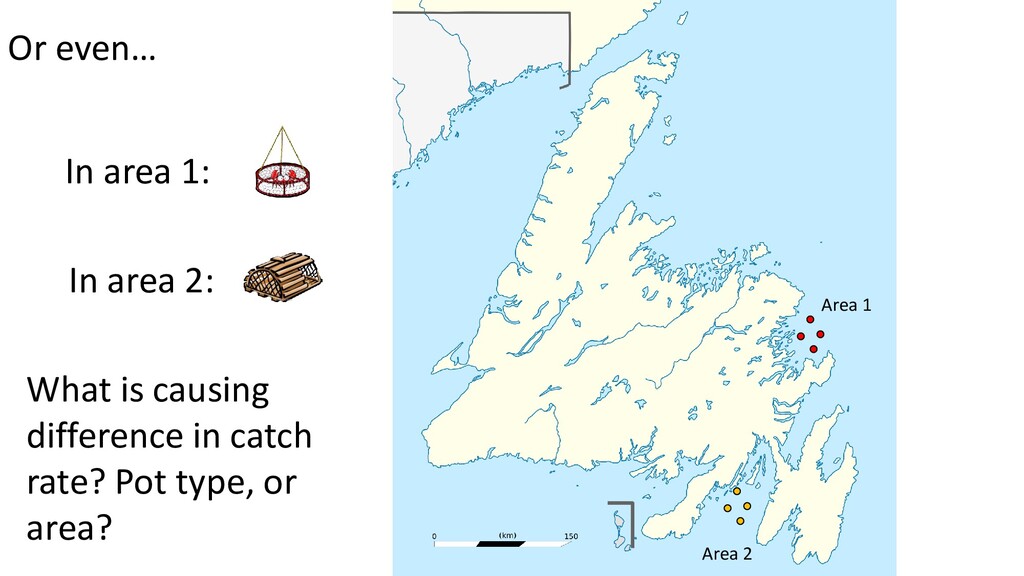
49. Collinearity X • Co-linearity of X values = X values vary together • Biological e.g.: Length and weight of fish (if both on X) • Experimental e.g.: Trap type and site Zuur et al (2009) http://onlinelibrary.wiley.com/doi/10.1111/j.2041-210X.2009.00001.x/full Good fishing site Bad site Here, site quality is collinear with trap type. They vary together. Another way to say this: As site changes, traps are also changing
50. “Correlation is not causation” could alternatively be said as: “We can’t be sure X1 affected Y, because X1 was correlated with X2 . We don’t know which was affecting Y” Good fishing site Bad site Is the blue site better? Or does it APPEAR better because we have better traps there?
51. Diameter Dataset on Urchin Size (Loi et al. 2017) Collinearity: Area x Site Size x Diameter Y: Gonad size (not here) X: Area, Site, Size class, diameter, Sex, Month
52. When should you be concerned? • Correlation > 0.8 always a disaster. Can only keep one in the model If X-Y relationship is very strong: - Correlation of 0.5-0.6 may be tolerable If X-Y relationship is weak: - Correlation even 0.3 to 0.4 can be a problem Careful! You can also have non-linear relationships between X values Check Variance Inflation Factor (VIF) score after modelling (later)
53. If covariate is a factor… Zuur and Ieno, (2016)
54. Zuur, Ieno, and Elphick (2010) Pre-exploration: Sketch out study design
55. Relationships X and Y • Plot Y versus each covariate Zuur et al (2010) http://onlinelibrary.wiley.com/doi/10.1111/j.2041-210X.2009.00001.x/full • Before you even run a model… do these relationships make sense? • One final check for entry errors Number of banded sparrows
56. Zuur, Ieno, and Elphick (2010) Pre-exploration: Sketch out study design
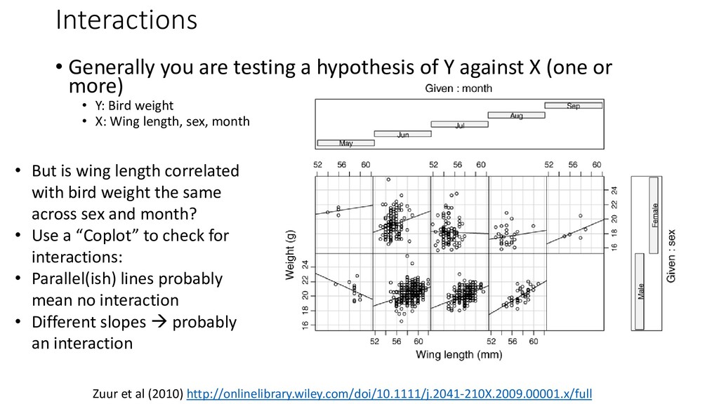
57. Interactions • Generally you are testing a hypothesis of Y against X (one or more) • Y: Bird weight • X: Wing length, sex, month Zuur et al (2010) http://onlinelibrary.wiley.com/doi/10.1111/j.2041-210X.2009.00001.x/full • But is wing length correlated with bird weight the same across sex and month? • Use a “Coplot” to check for interactions: • Parallel(ish) lines probably mean no interaction • Different slopes → probably an interaction
58. Zuur, Ieno, and Elphick (2010) Pre-exploration: Sketch out study design
59. Independence Y • See earlier slides… but once again: • Are values truly independent? • Spatially? • Temporally? • Nested experimental design? (Plants within garden plots? Pots within strings/fleets? Replications within Site?) • The answer is not always easy to determine. Think ecologically – how could my X values be influencing each other? Zuur et al (2009) http://onlinelibrary.wiley.com/doi/10.1111/j.2041-210X.2009.00001.x/full
60. Chapter 2: Data Exploration FISH 6003: Statistics and Study Design for Fisheries © Brett Favaro 2017 CatchRate ~ Poisson (μ ij ) E(CatchRate) = μ ij Log(μ ij ) = GearType ij + Temperature ij + FleetDeployment i FleetDeployment i ~ N(0, σ2) Using lme4: m <- glmer(CatchRate ~ GearType + Temperature + (1 | FleetDeployment), family = poisson) FISH 6003
61. Land Acknowledgment We would like to respectfully acknowledge the territory in which we gather as the ancestral homelands of the Beothuk, and the island of Newfoundland as the ancestral homelands of the Mi’kmaq and Beothuk. We would also like to recognize the Inuit of Nunatsiavut and NunatuKavut and the Innu of Nitassinan, and their ancestors, as the original people of Labrador. We strive for respectful partnerships with all the peoples of this province as we search for collective healing and true reconciliation and honour this beautiful land together. http://www.mun.ca/aboriginal_affairs/
62. Zuur, Ieno, and Elphick (2010) Pre-exploration: Sketch out study design
63. Your turn! Exercise time • Let’s do a data exploration on a paper with publicly-available data https://peerj.com/articl es/3067/
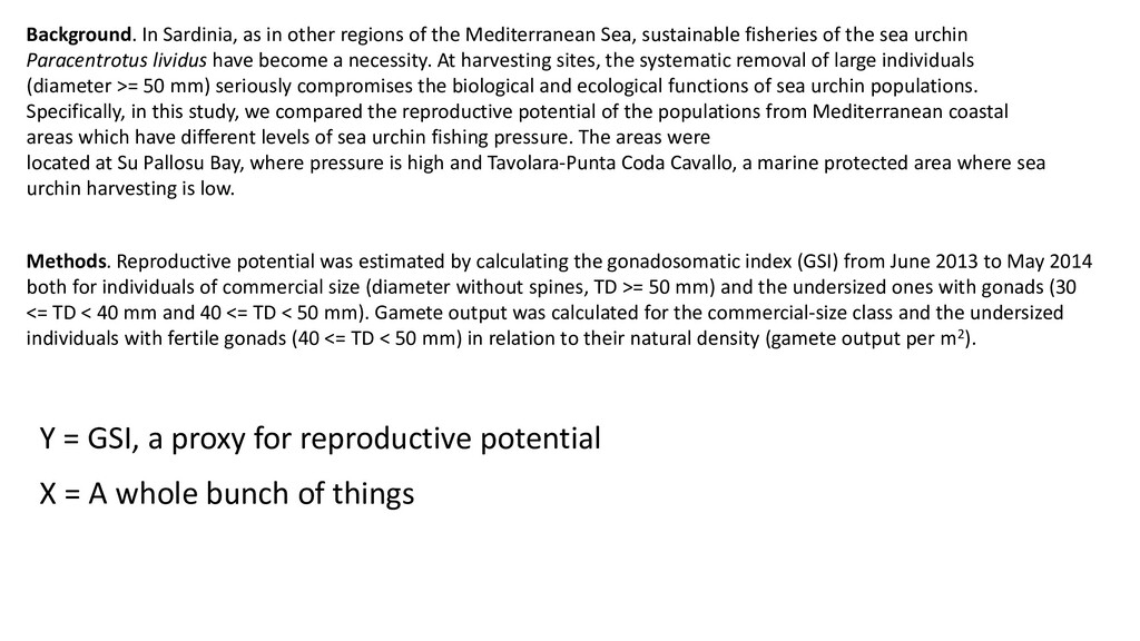
64. Background. In Sardinia, as in other regions of the Mediterranean Sea, sustainable fisheries of the sea urchin Paracentrotus lividus have become a necessity. At harvesting sites, the systematic removal of large individuals (diameter >= 50 mm) seriously compromises the biological and ecological functions of sea urchin populations. Specifically, in this study, we compared the reproductive potential of the populations from Mediterranean coastal areas which have different levels of sea urchin fishing pressure. The areas were located at Su Pallosu Bay, where pressure is high and Tavolara-Punta Coda Cavallo, a marine protected area where sea urchin harvesting is low. Methods. Reproductive potential was estimated by calculating the gonadosomatic index (GSI) from June 2013 to May 2014 both for individuals of commercial size (diameter without spines, TD >= 50 mm) and the undersized ones with gonads (30 <= TD < 40 mm and 40 <= TD < 50 mm). Gamete output was calculated for the commercial-size class and the undersized individuals with fertile gonads (40 <= TD < 50 mm) in relation to their natural density (gamete output per m2). Y = GSI, a proxy for reproductive potential X = A whole bunch of things
65. High Fishing Pressure (HP) Low Fishing Pressure (LP) Site
66. http://www.enchantedlearning.com/subjects/invertebrates/echinoderm/Seaurchin.shtml Test diameter … and some other things
67. First: Sketch the study design • 10 minutes to read paper, then we will draw together
68. I made two changes in Excel: 1. Assumed CreC was Area 2. Instead of having two tabs, I created a new column Site, and made it one big CSV file
69. Next: Open Week 2 R Project First: 001_DataSetup.R Second: 002_Exploration.R
70. Next: 003_MoreExploration.R
71. Final thoughts • Before you can run any model, you need to understand the data you’re working with • Often it requires major data cleanup – even before you start a formal data exploration. Never skip this, even with your own data! • You will make many decisions during a statistical analysis. Know WHY you made them. Write them down. You can always change your mind later • PeerJ is a good resource for experimental data in fisheries
72. Before we begin • Introducing MINOR ASSIGNMENT 1 http://derekogle.com/fishR/data/data- html/YERockfish.html Research question: Does age and length predict maturity stage? Before we can answer; Perform a data exploration
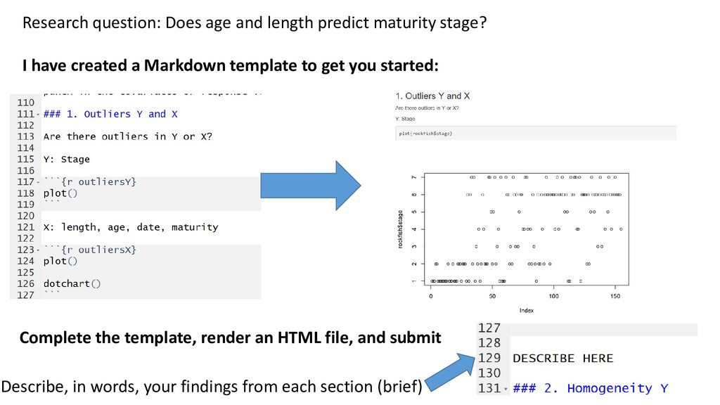
73. Research question: Does age and length predict maturity stage? I have created a Markdown template to get you started: Complete the template, render an HTML file, and submit Describe, in words, your findings from each section (brief)
74. Assignment value: 3 marks for each step of the data exploration (8 steps total) /1 All relevant variables are assessed at that step /1 Appropriate plots are used /1 Description of findings is defensible Total: /24, scaled to 10% of course grade Submit your HTML file into your OneDrive by Jan 30